Revisions to Combining histograms with a scatter plot

Commonmark migration

Source Link

edited Jun 16, 2020 at 9:23

Community Bot

1

###Sample data

Sample data

###Unframed with histograms sitting on the scatter plot frame

Unframed with histograms sitting on the scatter plot frame

Corrected errors in code

Source Link

edited Oct 19, 2017 at 13:53

m_goldberg

108.6k
16
107
263

histPlot1 = Histogram[histData1, 15, AspectRatio -> 1/5]; histPlot2 = Histogram[histData2, 12, AspectRatio -> 3, BarOrigin -> Left]; Framed[ Graphics[ {Text[Style["Plot Label", "SR", 16], Scaled@Scaled @ {.5, .96}], Inset[dataPlot, Scaled @ {.05, .03}, Scaled @ {0, 0}, Scaled[.73]], Inset[histPlot1, Scaled @ {.05, .77}, Scaled @ {0, 0}, Scaled[.7]], Inset[histPlot2, Scaled @ {.77, .03}, Scaled @ {0, 0}, Scaled[.75]]}, PlotRange -> MinMax /@ {histData1, histData2}, PlotRangePadding -> {{.01, .33}, {.0, .33}} /. u_Real -> Scaled[u], ImageSize -> {500, 450}]]

histPlot3 = Histogram[histData1, 15, AspectRatio -> 1/5, Ticks -> {None, Automatic}]; histPlot4 = Histogram[histData2, 12, AspectRatio -> 3, BarOrigin -> Left, Ticks -> {Automatic, None}]; Graphics[ {Text[Style["Plot Label", "SR", 16], Scaled@Scaled @ {.40, .96}], Inset[dataPlot, Scaled @ {.05, .03}, Scaled @ {0, 0}, Scaled[.77]], Inset[histPlot3, Scaled @ {.05, .76}, Scaled @ {0, 0}, Scaled[.7]], Inset[histPlot4, Scaled @ {.7645, .03}, Scaled @ {0, 0}, Scaled[.75]]}, PlotRange -> MinMax /@ {histData1, histData2}, PlotRangePadding -> {{.01, .33}, {.0, .33}} /. u_Real -> Scaled[u], ImageSize -> {500, 450}]

histPlot1 = Histogram[histData1, 15, AspectRatio -> 1/5]; histPlot2 = Histogram[histData2, 12, AspectRatio -> 3, BarOrigin -> Left]; Framed[ Graphics[ {Text[Style["Plot Label", 16], Scaled@{.5, .96}], Inset[dataPlot, Scaled @ {.05, .03}, Scaled @ {0, 0}, Scaled[.73]], Inset[histPlot1, Scaled @ {.05, .77}, Scaled @ {0, 0}, Scaled[.7]], Inset[histPlot2, Scaled @ {.77, .03}, Scaled @ {0, 0}, Scaled[.75]]}, PlotRange -> MinMax /@ {histData1, histData2}, PlotRangePadding -> {{.01, .33}, {.0, .33}} /. u_Real -> Scaled[u], ImageSize -> {500, 450}]]

histPlot3 = Histogram[histData1, 15, AspectRatio -> 1/5, Ticks -> {None, Automatic}]; histPlot4 = Histogram[histData2, 12, AspectRatio -> 3, BarOrigin -> Left, Ticks -> {Automatic, None}]; Graphics[ {Text[Style["Plot Label", 16], Scaled@{.40, .96}], Inset[dataPlot, Scaled @ {.05, .03}, Scaled @ {0, 0}, Scaled[.77]], Inset[histPlot3, Scaled @ {.05, .76}, Scaled @ {0, 0}, Scaled[.7]], Inset[histPlot4, Scaled @ {.7645, .03}, Scaled @ {0, 0}, Scaled[.75]]}, PlotRange -> MinMax /@ {histData1, histData2}, PlotRangePadding -> {{.01, .33}, {.0, .33}} /. u_Real -> Scaled[u], ImageSize -> {500, 450}]

histPlot1 = Histogram[histData1, 15, AspectRatio -> 1/5]; histPlot2 = Histogram[histData2, 12, AspectRatio -> 3, BarOrigin -> Left]; Framed[ Graphics[ {Text[Style["Plot Label", "SR", 16], Scaled @ {.5, .96}], Inset[dataPlot, Scaled @ {.05, .03}, Scaled @ {0, 0}, Scaled[.73]], Inset[histPlot1, Scaled @ {.05, .77}, Scaled @ {0, 0}, Scaled[.7]], Inset[histPlot2, Scaled @ {.77, .03}, Scaled @ {0, 0}, Scaled[.75]]}, PlotRange -> MinMax /@ {histData1, histData2}, PlotRangePadding -> {{.01, .33}, {.0, .33}} /. u_Real -> Scaled[u], ImageSize -> {500, 450}]]

histPlot3 = Histogram[histData1, 15, AspectRatio -> 1/5, Ticks -> {None, Automatic}]; histPlot4 = Histogram[histData2, 12, AspectRatio -> 3, BarOrigin -> Left, Ticks -> {Automatic, None}]; Graphics[ {Text[Style["Plot Label", "SR", 16], Scaled @ {.40, .96}], Inset[dataPlot, Scaled @ {.05, .03}, Scaled @ {0, 0}, Scaled[.77]], Inset[histPlot3, Scaled @ {.05, .76}, Scaled @ {0, 0}, Scaled[.7]], Inset[histPlot4, Scaled @ {.7645, .03}, Scaled @ {0, 0}, Scaled[.75]]}, PlotRange -> MinMax /@ {histData1, histData2}, PlotRangePadding -> {{.01, .33}, {.0, .33}} /. u_Real -> Scaled[u], ImageSize -> {500, 450}]

Corrected errors in code

Source Link

edited Oct 19, 2017 at 13:47

m_goldberg

108.6k
16
107
263

I prefer to use Graphics and Inset make this kind display figure. It requires a bit more work, but provides great flexibility in the placement of the elements. To illustrate the approach, I present two versions of your figure, The 1st is an arrangement that I personally find pleasing; the 2nd is closer to what you show in your question.

###Sample data

SeedRandom[1]; data = RandomReal[BinormalDistribution[{0, 0}, {1, 1}, 0.5], 50]; {histData1, histData2} = Transpose @ data; dataPlot = Graphics[Point @ data, Frame -> True];

Framed with full axes data

histPlot1 = Histogram[histData1, 15, AspectRatio -> 1/5]; histPlot2 = Histogram[histData2, 12, AspectRatio -> 3, BarOrigin -> Left]; Framed[ Graphics[ {Text[Style["Plot Label", 16], Scaled@{.5, .96}], Inset[dataPlot, Scaled @ {.05, .03}, Scaled @ {0, 0}, Scaled[.73]], Inset[histPlot1, Scaled @ {.05, .77}, Scaled @ {0, 0}, Scaled[.7]], Inset[histPlot2, Scaled @ {.77, .03}, Scaled @ {0, 0}, Scaled[.75]]}, PlotRange -> MinMax /@ {histData1, histData2}, PlotRangePadding -> {{.01, .33}, {.0, .33}} /. u_Real -> Scaled[u], ImageSize -> {500, 450}]]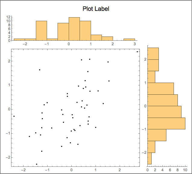

###Unframed with histograms sitting on the scatter plot frame

histPlot3 = Histogram[histData1, 15, AspectRatio -> 1/5, Ticks -> {None, Automatic}]; histPlot2histPlot4 = Histogram[histData2, 12, AspectRatio -> 3, BarOrigin -> Left, Ticks -> {Automatic, None}]; Graphics[ {Text[Style["Plot Label", 16], Scaled@{.40, .96}], Inset[dataPlot, Scaled @ {.05, .03}, Scaled @ {0, 0}, Scaled[.77]], Inset[histPlot3, Scaled @ {.05, .76276}, Scaled @ {0, 0}, Scaled[.7]], Inset[histPlot2Inset[histPlot4, Scaled @ {.7645, .03}, Scaled @ {0, 0}, Scaled[.75]]}, PlotRange -> MinMax /@ {histData1, histData2}, PlotRangePadding -> {{.01, .33}, {.0, .33}} /. u_Real -> Scaled[u], ImageSize -> {500, 450}]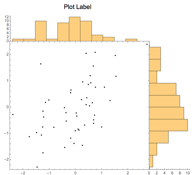

Even if neither of these figures is exactly what you are looking for, I think these examples show the versatility this approach. I hope you can adapt to your needs.

I prefer to use Graphics and Inset make this kind display figure. It requires a bit more work, but provides great flexibility in the placement of the elements. To illustrate the approach, I present two versions of your figure, The 1st is an arrangement that I personally find pleasing; the 2nd is closer to what you show in your question.

###Sample data

SeedRandom[1]; data = RandomReal[BinormalDistribution[{0, 0}, {1, 1}, 0.5], 50]; {histData1, histData2} = Transpose @ data; dataPlot = Graphics[Point @ data, Frame -> True];

Framed with full axes data

histPlot1 = Histogram[histData1, 15, AspectRatio -> 1/5]; histPlot2 = Histogram[histData2, 12, AspectRatio -> 3, BarOrigin -> Left]; Framed[ Graphics[ {Text[Style["Plot Label", 16], Scaled@{.5, .96}], Inset[dataPlot, Scaled @ {.05, .03}, Scaled @ {0, 0}, Scaled[.73]], Inset[histPlot1, Scaled @ {.05, .77}, Scaled @ {0, 0}, Scaled[.7]], Inset[histPlot2, Scaled @ {.77, .03}, Scaled @ {0, 0}, Scaled[.75]]}, PlotRange -> MinMax /@ {histData1, histData2}, PlotRangePadding -> {{.01, .33}, {.0, .33}} /. u_Real -> Scaled[u], ImageSize -> {500, 450}]]

###Unframed with histograms sitting on the scatter plot frame

histPlot3 = Histogram[histData1, 15, AspectRatio -> 1/5, Ticks -> {None, Automatic}]; histPlot2 = Histogram[histData2, 12, AspectRatio -> 3, BarOrigin -> Left, Ticks -> {Automatic, None}]; Graphics[ {Text[Style["Plot Label", 16], Scaled@{.40, .96}], Inset[dataPlot, Scaled @ {.05, .03}, Scaled @ {0, 0}, Scaled[.77]], Inset[histPlot3, Scaled @ {.05, .762}, Scaled @ {0, 0}, Scaled[.7]], Inset[histPlot2, Scaled @ {.7645, .03}, Scaled @ {0, 0}, Scaled[.75]]}, PlotRange -> MinMax /@ {histData1, histData2}, PlotRangePadding -> {{.01, .33}, {.0, .33}} /. u_Real -> Scaled[u], ImageSize -> {500, 450}]

Even if neither of these figures is exactly what you are looking for, I think these examples show the versatility this approach. I hope you can adapt to your needs.

I prefer to use Graphics and Inset make this kind display figure. It requires a bit more work, but provides great flexibility in the placement of the elements. To illustrate the approach, I present two versions of your figure, The 1st is an arrangement that I personally find pleasing; the 2nd is closer to what you show in your question.

###Sample data

SeedRandom[1]; data = RandomReal[BinormalDistribution[{0, 0}, {1, 1}, 0.5], 50]; {histData1, histData2} = Transpose @ data; dataPlot = Graphics[Point @ data, Frame -> True];

Framed with full axes data

histPlot1 = Histogram[histData1, 15, AspectRatio -> 1/5]; histPlot2 = Histogram[histData2, 12, AspectRatio -> 3, BarOrigin -> Left]; Framed[ Graphics[ {Text[Style["Plot Label", 16], Scaled@{.5, .96}], Inset[dataPlot, Scaled @ {.05, .03}, Scaled @ {0, 0}, Scaled[.73]], Inset[histPlot1, Scaled @ {.05, .77}, Scaled @ {0, 0}, Scaled[.7]], Inset[histPlot2, Scaled @ {.77, .03}, Scaled @ {0, 0}, Scaled[.75]]}, PlotRange -> MinMax /@ {histData1, histData2}, PlotRangePadding -> {{.01, .33}, {.0, .33}} /. u_Real -> Scaled[u], ImageSize -> {500, 450}]]

###Unframed with histograms sitting on the scatter plot frame

histPlot3 = Histogram[histData1, 15, AspectRatio -> 1/5, Ticks -> {None, Automatic}]; histPlot4 = Histogram[histData2, 12, AspectRatio -> 3, BarOrigin -> Left, Ticks -> {Automatic, None}]; Graphics[ {Text[Style["Plot Label", 16], Scaled@{.40, .96}], Inset[dataPlot, Scaled @ {.05, .03}, Scaled @ {0, 0}, Scaled[.77]], Inset[histPlot3, Scaled @ {.05, .76}, Scaled @ {0, 0}, Scaled[.7]], Inset[histPlot4, Scaled @ {.7645, .03}, Scaled @ {0, 0}, Scaled[.75]]}, PlotRange -> MinMax /@ {histData1, histData2}, PlotRangePadding -> {{.01, .33}, {.0, .33}} /. u_Real -> Scaled[u], ImageSize -> {500, 450}]

Even if neither of these figures is exactly what you are looking for, I think these examples show the versatility this approach. I hope you can adapt to your needs.