Return to Answer

For illustrative purposes, we will consider a circular boundary (note that this can easily be put turned into a single Boolean function using polar coordinates, but there are many perfectly nice space curves that cannot):

Nt = 10; Rf = 2;(* Resampling factor *) Stf = 1/4;(* Scafolding thickness factor *) 

For illustrative purposes, we will consider a circular boundary (note that this can easily be turned into a single Boolean function using polar coordinates, but there are many perfectly nice space curves that cannot):

Nt = 10; Rf = 2;(* Resampling factor *) Stf = 1/2;(* Scafolding thickness factor *) 

Nt = 10; Rf = 2;(* Resampling factor *) 

coordsOuter = {}; coordsInner = {}; For[i = 1, i <= Nt, i++, l = (Norm[Bcoords[[ci[i, Nt]]] - Bcoords[[ci[i - 1, Nt]]]] + Norm[Bcoords[[ci[i + 1, Nt]]] - Bcoords[[ci[i, Nt]]]])/4; (* choose size of scaffolding similar to distance to neighboring points *) tv = tanVecs[[i]]; n = {tv[[2]], -tv[[1]]};(* n = t x Overscript[z, ^] *) AppendTo[coordsOuter, Bcoords[[i]] + l n]; AppendTo[coordsInner, Bcoords[[i]] - l n]; ]; 

Nt = 10; Rf = 2;(* Resampling factor *) Stf = 1/4;(* Scafolding thickness factor *) 

coordsOuter = {}; coordsInner = {}; For[i = 1, i <= Nt, i++, l = Stf (Norm[Bcoords[[ci[i, Nt]]] - Bcoords[[ci[i - 1, Nt]]]] + Norm[Bcoords[[ci[i + 1, Nt]]] - Bcoords[[ci[i, Nt]]]])/2; (* choose size of scaffolding using distance to neighboring points *) tv = tanVecs[[i]]; n = {tv[[2]], -tv[[1]]};(* n = t x Overscript[z, ^] *) AppendTo[coordsOuter, Bcoords[[i]] + l n]; AppendTo[coordsInner, Bcoords[[i]] - l n]; ]; 

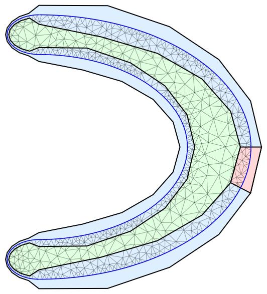
EDIT: Here a nontrivial space curve to demonstrate the method works generally.

xyE[θ_, el_] := {el Cos[θ], Sin[θ]}; xy[t_, wf_, el_] := Module[{θ}, Which[ 0 <= t < Pi/2, θ = 2 t - Pi/2; xyE[θ, el], Pi/2 <= t < Pi, θ = 2 t - Pi/2; (1 - wf)/2 xyE[θ, el] + {0, (1 + wf)/2}, Pi <= t < 3 Pi/2, θ = 5 Pi/2 - 2 t; wf xyE[θ, el], 3 Pi/2 <= t <= 2 Pi, θ = 2 t - 5 Pi/2; (1 - wf)/2 xyE[θ, el] - {0, (1 + wf)/2} ] ]; xyEP[θ_, el_] := {-el Sin[θ], Cos[θ]}; xyP[t_, wf_, el_] := Module[{θ}, Which[ 0 <= t < Pi/2, θ = 2 t - Pi/2; 2 xyEP[θ, el], Pi/2 <= t < Pi, θ = 2 t - Pi/2; 2 (1 - wf)/2 xyEP[θ, el], Pi <= t < 3 Pi/2, θ = 5 Pi/2 - 2 t; -2 wf xyEP[θ, el], 3 Pi/2 <= t <= 2 Pi, θ = 2 t - 5 Pi/2; 2 (1 - wf)/2 xyEP[θ, el] ] ]; wf = 0.7; el = 1.6; xy[t_] := xy[t, wf, el]; xyP[t_] := xyP[t, wf, el]; 

Set global parameters

Nt = 40; Rf = 3;(* Resampling factor *) Stf = 1/4;(* Scafolding thickness factor *) 

Visualize the result like before:

ii = 5; Show[ Graphics[{{EdgeForm[Thick], LightBlue, POuter}, {EdgeForm[Thick], LightGreen, PInner}, {EdgeForm[Thick], LightRed, getPoly[ii, ii]}}], ParametricPlot[xy[t], {t, 0, 2 Pi}, Axes -> False, PlotStyle -> Blue], meshS["Wireframe"["MeshElementStyle" -> EdgeForm[Thin]]]] 

Define the global function to give to.

Fixing N_t = 10, we vary Rf. A polygonal mesh is built for comparison

In[501]:= SError Out[501]= {{2, 0.00330491}, {4, 0.000206049}, {8, 0.0000128467}, {16, 7.98742*10^-7}} In[502]:= PError Out[502]= {{2, 0.0514227}, {4, 0.0129034}, {8, 0.00322882}, {16, 0.000807393}} FitP = Table[{PError[[i, 1]], PError[[1, 2]] (PError[[i, 1]]/PError[[1, 1]])^-2}, {i, 1, Length[PError]}]; FitS = Table[{SError[[i, 1]], SError[[1, 2]] (SError[[i, 1]]/SError[[1, 1]])^-4}, {i, 1, Length[SError]}]; ListLogLogPlot[{SError, FitS, PError, FitP}, Joined -> {False, True, False, True}] 

Define the global function to give to ImplicitRegion.

Fixing Nt = 10, we vary Rf. A polygonal mesh is built for comparison

SError 

{{2, 0.00330491}, {4, 0.000206049}, {8, 0.0000128467}, {16, 7.98742*10^-7}}

PError 

{{2, 0.0514227}, {4, 0.0129034}, {8, 0.00322882}, {16, 0.000807393}}

FitP = Table[{PError[[i, 1]], PError[[1, 2]] (PError[[i, 1]]/PError[[1, 1]])^-2}, {i, 1, Length[PError]}]; FitS = Table[{SError[[i, 1]], SError[[1, 2]] (SError[[i, 1]]/SError[[1, 1]])^-4}, {i, 1, Length[SError]}]; ListLogLogPlot[{SError, FitS, PError, FitP}, Joined -> {False, True, False, True}]