You could use an image representation of the plot and map it onto the modified cylinder that I defined in the answer linked herethe answer linked here.
replaced http://mathematica.stackexchange.com/ with https://mathematica.stackexchange.com/
To combine transparency with a cylinder "backbone" for better visibility, you could do it like this:
Graphics3D[{Texture[ImageData@img], EdgeForm[], cyl[{{0, 0, 0}, {0, 0, 2 Pi}}, 1], FaceForm[Directive[Opacity[.5], Orange]], Cylinder[{{0, 0, -.01}, {0, 0, 2 Pi + .01}}, .99]}, Boxed -> False, Lighting -> "Neutral"] 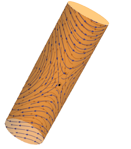
To combine transparency with a cylinder "backbone" for better visibility, you could do it like this:
Graphics3D[{Texture[ImageData@img], EdgeForm[], cyl[{{0, 0, 0}, {0, 0, 2 Pi}}, 1], FaceForm[Directive[Opacity[.5], Orange]], Cylinder[{{0, 0, -.01}, {0, 0, 2 Pi + .01}}, .99]}, Boxed -> False, Lighting -> "Neutral"]
You could use an image representation of the plot and map it onto the modified cylinder that I defined in the answer linked here.
Just copy the definition of cyl from that answer, which includes the ability to add textures as follows:
img = Image@StreamPlot[{y, -Sin[x]}, {x, -5, 5}, {y, -3, 3}, Frame -> None, PlotRange -> {{-5, 5}, {-3, 3}}, Epilog -> {PointSize -> Large, Point[{{0, 0}, {Pi, 0}, {-Pi, 0}}]}, StreamPoints -> Fine, AspectRatio -> 0.8, PlotRangePadding -> 0, ImageMargins -> 0, ImageSize -> 800]; Graphics3D[{Texture[img], EdgeForm[], cyl[{{0, 0, 0}, {0, 0, 2 Pi}}, 1]}, Boxed -> False] 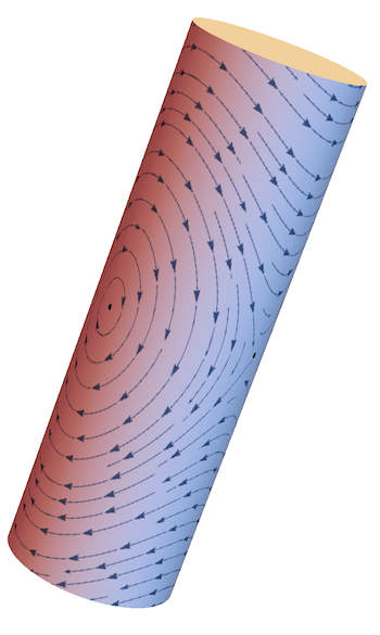
The resolution is controlled by the options of Image or by the ImageSize options in StreamPlot.
I also added the PlotRange to the original plot to suppress the plot range padding.
Edit
To make the whole thing transparent, you can use the same approach provided that the image has an alpha channel with transparent background:
img = Rasterize[ StreamPlot[{y, -Sin[x]}, {x, -5, 5}, {y, -3, 3}, Frame -> None, PlotRange -> {{-5, 5}, {-3, 3}}, Epilog -> {PointSize -> Large, Point[{{0, 0}, {Pi, 0}, {-Pi, 0}}]}, StreamPoints -> Fine, AspectRatio -> 0.8, PlotRangePadding -> 0, ImageMargins -> 0, ImageSize -> 500], Background -> None, ImageResolution -> 300 ]; Graphics3D[{Texture[ImageData@img], EdgeForm[], cyl[{{0, 0, 0}, {0, 0, 2 Pi}}, 1]}, Boxed -> False, Lighting -> "Neutral"] 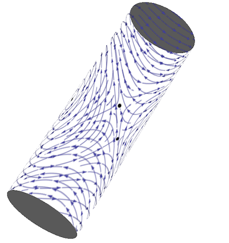
Here I used Rasterize because it permits a Background -> None option. Also, I used ImageResolution in combination with the ImageSize specification of the StreamPlot to make sure that the Points from the Epilog in the original plot are properly visible.
You could use an image representation of the plot and map it onto the modified cylinder that I defined in the answer.
Just copy the definition of cyl from that answer, which includes the ability to add textures as follows:
img = Image@StreamPlot[{y, -Sin[x]}, {x, -5, 5}, {y, -3, 3}, Frame -> None, PlotRange -> {{-5, 5}, {-3, 3}}, Epilog -> {PointSize -> Large, Point[{{0, 0}, {Pi, 0}, {-Pi, 0}}]}, StreamPoints -> Fine, AspectRatio -> 0.8, PlotRangePadding -> 0, ImageMargins -> 0, ImageSize -> 800]; Graphics3D[{Texture[img], EdgeForm[], cyl[{{0, 0, 0}, {0, 0, 2 Pi}}, 1]}, Boxed -> False]
The resolution is controlled by the options of Image or by the ImageSize options in StreamPlot.
I also added the PlotRange to the original plot to suppress the plot range padding.
You could use an image representation of the plot and map it onto the modified cylinder that I defined in the answer linked here.
Just copy the definition of cyl from that answer, which includes the ability to add textures as follows:
img = Image@StreamPlot[{y, -Sin[x]}, {x, -5, 5}, {y, -3, 3}, Frame -> None, PlotRange -> {{-5, 5}, {-3, 3}}, Epilog -> {PointSize -> Large, Point[{{0, 0}, {Pi, 0}, {-Pi, 0}}]}, StreamPoints -> Fine, AspectRatio -> 0.8, PlotRangePadding -> 0, ImageMargins -> 0, ImageSize -> 800]; Graphics3D[{Texture[img], EdgeForm[], cyl[{{0, 0, 0}, {0, 0, 2 Pi}}, 1]}, Boxed -> False]
The resolution is controlled by the options of Image or by the ImageSize options in StreamPlot.
I also added the PlotRange to the original plot to suppress the plot range padding.
Edit
To make the whole thing transparent, you can use the same approach provided that the image has an alpha channel with transparent background:
img = Rasterize[ StreamPlot[{y, -Sin[x]}, {x, -5, 5}, {y, -3, 3}, Frame -> None, PlotRange -> {{-5, 5}, {-3, 3}}, Epilog -> {PointSize -> Large, Point[{{0, 0}, {Pi, 0}, {-Pi, 0}}]}, StreamPoints -> Fine, AspectRatio -> 0.8, PlotRangePadding -> 0, ImageMargins -> 0, ImageSize -> 500], Background -> None, ImageResolution -> 300 ]; Graphics3D[{Texture[ImageData@img], EdgeForm[], cyl[{{0, 0, 0}, {0, 0, 2 Pi}}, 1]}, Boxed -> False, Lighting -> "Neutral"]
Here I used Rasterize because it permits a Background -> None option. Also, I used ImageResolution in combination with the ImageSize specification of the StreamPlot to make sure that the Points from the Epilog in the original plot are properly visible.