How can I find the points where these two graphs intersect:
ContourPlot[{x == 1/2 (1 + Tanh[(x y^2)/0.5]),y == Tanh[(x^2 y)/0.5]}, {x, 0, 2}, {y, -1, 1}] 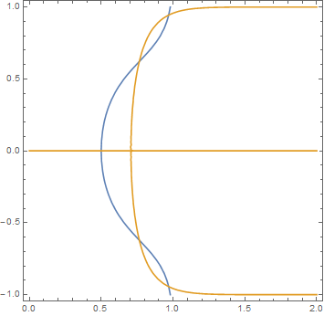
How can I find the points where these two graphs intersect:
ContourPlot[{x == 1/2 (1 + Tanh[(x y^2)/0.5]),y == Tanh[(x^2 y)/0.5]}, {x, 0, 2}, {y, -1, 1}]
FindRoot is the first thing that comes to mind with this type of problems. First, create a list of initial conditions for the root search, based on the plot (rough estimates are sufficient):
init = {{0.5, 0}, {0.75, 0.75}, {0.75, -0.75}, {1, 1}, {1, -1}}; Make a pure function that will find the roots:
f = FindRoot[{x == 1/2 (1 + Tanh[(x y^2)/0.5]), y == Tanh[(x^2 y)/0.5]}, {{x, #1}, {y, #2}}] & and apply it to the initial conditions:
roots = f @@@ init {{x -> 0.5, y -> 0.}, {x -> 0.764865, y -> 0.620918}, {x -> 0.764865, y -> -0.620918}, {x -> 0.969417, y -> 0.944097}, {x -> 0.969417, y -> -0.944097}}
or just
{x, y} /. roots {{0.5, 0.}, {0.764865, 0.620918}, {0.764865, -0.620918}, {0.969417, 0.944097}, {0.969417, -0.944097}}
EDIT: I developed a different method, suitable for this problem also, while answering another question.
Let's take the plot in the form
curve = ContourPlot[{x == 1/2 (1 + Tanh[(x y^2)/0.5]), y == Tanh[(x^2 y)/0.5]}, {x, 0, 2}, {y, -1, 1}, Frame -> None, PlotRangePadding -> None] and extract the pixel positions of intersection with
px = PixelValuePositions[#, White] & @ MorphologicalBranchPoints @ Thinning @ Binarize @ ColorNegate @ curve We need to connect them to the actual coordinates on the plot:
pl = PlotRange@curve {{0., 2.}, {-1., 1.}}
id = ImageDimensions@curve {360, 360}
The relation between pl and id is linear, $y=ax+b$ and $y=cx+d$ in the horizontal and vertical directions, respecively:
{a, b} = {a, b} /. First@Solve[{pl[[1, 1]] == b, pl[[1, 2]] == a id[[1]] + b}, {a, b}] {c, d} = {c, d} /. First@Solve[{pl[[2, 1]] == d, pl[[2, 2]] == c id[[2]] + d}, {c, d}] {0.00555556, 0.}
{0.00555556, -1.}
The pixel positions transformed to plot coordinates:
ic = {a #1 + b, c #2 + d} & @@@ px {{0.983333, 0.961111}, {0.988889, 0.955556}, {0.977778, 0.95}, {0.961111, 0.933333}, {0.783333, 0.638889}, {0.761111, 0.605556}, {0.755556, 0.6}, {0.761111, 0.594444}, {0.505556, 0.}, {0.711111, 0.}, {0.716667, 0.}, {0.761111, -0.594444}, {0.755556, -0.6}, {0.761111, \ -0.605556}, {0.777778, -0.638889}, {0.961111, -0.933333}, {0.977778, \ -0.95}}
look like this:
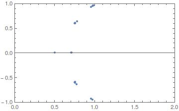
Not exactly at the intersections, but this is good enough. We can get rid of the ambiguity with clustering:
clu = ClusterClassify[ic, Method -> "DBSCAN"] Number of clusters: 6
g = GatherBy[ic, clu] icmean = Reverse[Mean /@ g] {{0.969444, -0.941667}, {0.763889, -0.609722}, {0.713889, 0.}, {0.505556, 0.}, {0.765278, 0.609722}, {0.977778, 0.95}}
Show[curve, Graphics[{PointSize[Large], Point[#]}] &@icmean] 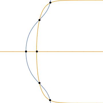
which looks very good. The additional intersection of the orange curve with itself was found additinally.
MeshFunctionsone can directly plot the solution with a "one-liner"ContourPlot[{f[x, y], g[x, y]}, {x, 0, 2}, {y, -1, 1}, MeshFunctions -> {f[#1, #2] - g[#1, #2] &}, Mesh -> {{0}}, MeshStyle -> Directive[Red, PointSize[Large]]]$\endgroup$