7
$\begingroup$

An example, the command

DSolve[y''[x] - 4 y[x] == 1, y[x], x] 

gives solution

y[x] -> -(1/4) + E^(2 x) C[1] + E^(-2 x) C[2] 

The same command with initial conditions

DSolve[{y''[x] - 4 y[x] == 1, y[0] == 1, y'[1] == -1}, y[x], x] 

gives solution

y[x] -> -((E^(-2 x) (-2 E^2 - 5 E^4 + E^(2 x) - 5 E^(4 x) + E^(4 + 2 x) + 2 E^(2 + 4 x)))/(4 (1 + E^4))) 

In the first case, the solution has very clear structure: an increasing component, a decreasing component, and a particular solution. In the second case, this structure is shadowed by the complicated expression. Here is a picture of the commands & results in Mathematica:

snapshot

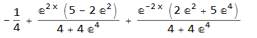
I think most people would prefer the 2nd solution to be presented in similar form as in the first case. Something like:

The solution is $y = c_1 h_1(x) + c_2 h_2(x) + g(x)$, in which $h_1(x) = e^{2 x}$ is the first homogeneous solution, $h_2(x) = e^{-2 x}$ is the second homogeneous solution, and $g(x)=-1/4$ is the particular solution. The coefficients $c_1, c_2$ are determined from initial conditions. In this particular case we have $ c_1 = ; c_2 = $.

Is there a way to extract $c_1$ and $c_2$? Pattern matching might work in this simple example, but I don't think it generalizes to more complicated cases.

$\endgroup$
0

8 Answers 8

8
$\begingroup$

It's possible to dig out C[_] directly from DSolve, with the help of TraceInternal:

eqn = y''[x] - 4 y[x] == 1; constant = Trace[DSolve[{eqn, y[0] == 1, y'[1] == -1}, y[x], x], HoldPattern[C[_] -> _], TraceInternal -> True] // Flatten // ReleaseHold // Simplify // Union (* {C[1] -> (5 - 2 E^2)/(4 + 4 E^4), C[2] -> (2 E^2 + 5 E^4)/(4 + 4 E^4)} *) 

Or a bit shorter:

constant = Trace[DSolve[{eqn, y[0] == 1, y'[1] == -1}, y[x], x], HoldPattern[{(C[_] -> _) ..}], TraceInternal -> True] // ReleaseHold // Flatten 
$\endgroup$
6
$\begingroup$

The most obvious answer is to solve for the constants from the general solution directly. In this example, let

gensol = DSolve[y''[x] - 4 y[x] == 1, y[x], x][[1, 1, 2]] (*-(1/4) + E^(2 x) C[1] + E^(-2 x) C[2]*) 

Now we can construct a system of equations based on the boundary conditions specified in the problem to get explicit values for our general solution constants.

FullSimplify@ Solve[{Evaluate[gensol /. x -> 0] == 1, Evaluate[D[gensol, x] /. x -> 1] == -1}, {C[1], C[2]}] (*{{C[1] -> (5 - 2 E^2)/(4 + 4 E^4), C[2] -> (2 E^2 + 5 E^4)/(4 + 4 E^4)}}*) 

In this example we also mess around a bit with the full solution to extract the general solution constants.

totsol = DSolve[{y''[x] - 4 y[x] == 1, y[0] == 1, y'[1] == -1}, y[x], x][[1, 1, 2]] (*-((E^(-2 x) (-2 E^2 - 5 E^4 + E^(2 x) - 5 E^(4 x) + E^(4 + 2 x) + 2 E^(2 + 4 x)))/(4 (1 + E^4)))*) 

Collecting the results based on one of the functions appearing in the general solution we can extract the constants.

Collect[Expand[totsol], E^(2 x)] (*-(1/(4 (1 + E^4))) - E^4/(4 (1 + E^4)) + E^(2 x) (5/(4 (1 + E^4)) - E^2/(2 (1 + E^4))) + E^(-2 x) (E^2/(2 (1 + E^4)) + (5 E^4)/(4 (1 + E^4)))*) 

We can now simplify things a bit to get the constants.

FullSimplify[-(1/(4 (1 + E^4))) - E^4/(4 (1 + E^4))] (*-(1/4)*) FullSimplify[{(5/(4 (1 + E^4)) - E^2/(2 (1 + E^4))), (E^2/( 2 (1 + E^4)) + (5 E^4)/(4 (1 + E^4)))}] (*{(5 - 2 E^2)/(4 + 4 E^4), (2 E^2 + 5 E^4)/(4 + 4 E^4)}*) 

Checking that we get the same answer in both methods:

FullSimplify[{(5/(4 (1 + E^4)) - E^2/(2 (1 + E^4))), (E^2/( 2 (1 + E^4)) + (5 E^4)/(4 (1 + E^4)))}] == Flatten@FullSimplify@ Solve[{Evaluate[gensol /. x -> 0] == 1, Evaluate[D[gensol, x] /. x -> 1] == -1}, {C[1], C[2]}][[;; , ;; , 2]] (*True*) 
$\endgroup$
2
  • $\begingroup$ Same idea, slightly different functions/usage: foo = Collect[Expand[totsol], E^(2 x), Simplify], Simplify@Coefficient[foo, {E^(2 x), E^(-2 x)}], Coefficient[foo, {E^(2 x)}, 0] $\endgroup$ Commented Apr 4, 2017 at 20:30
  • $\begingroup$ Actually Evaluate isn't necessary, you can simply use parentheses or e.g. gensol == 1 /. x -> 0 $\endgroup$ Commented Apr 5, 2017 at 7:26
4
$\begingroup$

If you do it the following way, applying the shown rules, you get the desired result.

This can be used for all types of equations.

 dsol = First@DSolve[y''[x] - 4 y[x] == 1, y, x] (* {y -> Function[{x}, -(1/4) + E^(2 x) C[1] + E^(-2 x) C[2]]} *) sol = First@Solve[{y[0] == a, y'[0] == b} /. dsol, {C[1], C[2]}] (* {C[1] -> 1/8 (1 + 4 a + 2 b), C[2] -> 1/8 + a/2 - b/4} *) ys[x_, a_, b_] = (y[x] /. dsol /. sol) (* -(1/4) + (1/8 + a/2 - b/4) E^(-2 x) + 1/8 (1 + 4 a + 2 b) E^(2 x) *) 
$\endgroup$
1
  • $\begingroup$ @ xzczd you are right. You get the same effect without Unevaluated. Then this is the solution without Unevaluated. $\endgroup$ Commented Apr 5, 2017 at 6:40
3
$\begingroup$

Once defined the following function:

dsolve[ode_, ic_, fun_, var_] := Module[{constant, i}, fun = DSolve[ode, fun, var][[1, 1, 2]]; constant = Table[C[i], {i, 1, Length[ic]}]; constant = Solve[ic, constant]; For[i = 1, i <= Length[ic], i++, fun = fun /. C[i] -> constant[[1, i, 2]] ]; Return[fun[[2]]]]; 

writing:

Clear[y] ode = y''[x] - 4 y[x] == 1; ic = {y[0] == 1, y'[1] == -1}; dsolve[ode, ic, y, x] 

you get:

-(1/4) - (E^(2 x) (-5 + 2 E^2))/(4 (1 + E^4)) - (E^(-2 x) (-2 E^2 - 5 E^4))/(4 (1 + E^4)) 

which is as much as desired.

$\endgroup$
1
  • $\begingroup$ I'm sorry, but this function isn't that… good. Let alone the redundant Return and unnecessary For, the most serious issue is, fun will be polluted. Just try executing dsolve[ode, ic, y, x] twice. A possible countermeasure is to introduce another intermediate variable in Module. $\endgroup$ Commented Apr 5, 2017 at 8:24
3
$\begingroup$

SolveAlways cannot handle the mixed forms E^(2 + 4 x), E^(4 x), etc., but a change of variables fixes that.

gensol = First@DSolve[y''[x] - 4 y[x] == 1, y[x], x]; partsol = First@DSolve[{y''[x] - 4 y[x] == 1, y[0] == 1, y'[1] == -1}, y[x], x]; SolveAlways[(y[x] /. gensol) == (y[x] /. partsol) /. x -> Log@u, u] (* {{C[1] -> (5 - 2 E^2)/(4 (1 + E^4)), C[2] -> (2 E^2 + 5 E^4)/(4 (1 + E^4))}} *) 
$\endgroup$
3
$\begingroup$

This works:

DSolve[{y''[x] - 4 y[x] == 1, y[0] == 1, y'[1] == -1}, y[x], x] // Collect[#, E^(2 x)] & 

enter image description here

$\endgroup$
3
$\begingroup$

Another form with a compact structure is

soln = First@DSolve[ {y''[x] - 4 y[x] == 1, y[0] == 1, y'[1] == -1}, y[x], x]; soln // ExpToTrig // FullSimplify 

enter image description here

$\endgroup$
3
$\begingroup$

Here is another way to find C's

eqn = y''[x] - 4 y[x] == 1; s = DSolve[eqn, y[x], x]; gsol[x_] = y[x] /. Flatten[s]; dgsol[x_] = D[y[x] /. Flatten[s], x]; findCs = Solve[{gsol[0] == 1, dgsol[1] == -1}, {C[1], C[2]}]// Simplify 

enter image description here

gsol[x] /. Flatten[findCs] 

enter image description here

Simplify[eqn /. {{y[x] -> %}} /. {{y''[x] -> D[%, x, x]}}] 

{{True}}

$\endgroup$
0

Start asking to get answers

Find the answer to your question by asking.

Ask question

Explore related questions

See similar questions with these tags.