It seems that the modeling of the step input for the current is rather not physical. The invariant is delayed perturbed in a non-neglectable manner.
First, take into account that NDSolve is proven in practice and not a built-in that is made for step size control. That was a wish by the Mathematica customers and a consequence of the test suits on which it is verified for the highest possible versatility. It saves time and effort for the users.
There are still of course workarounds to control step size for tedious and error-prone partial differential equations. This case is not close to such problems.
I did put the precision options out of the command. Automatic means for the Projection option too the use of Runge-Kutta. A proper choice for it is to match the order of the coefficients favored. So with Automatic these whole lot of optimization are done by Mathematica in NDSolve for the best solution.
With this in mind the results for
Remove["Global`*"] (*PARAMETERS*) γ = 1.76*10.^7*10.^4 (*T^-1s^-1*); α = 0.06; θsh = 0.3; Ms \ = 7.*10.^5;(*A/m*)tFM = 2.*10.^-9;(*m*)currAMP = 30.*10.^-3 (*A*); sHM = 10.*10.^-6*3.*10.^-9(*m^2,tHM=3 nm*); Hamp = 0.03; Hk = 0.1; a = 0. °; b = 0. °; c = 0. °; Ang = 0. °; temp = 3; rad = 20.*10.^-9;(*Thermal effect*)kTL = 2.; tSt = 0.; tFin = 1.5*10.0^-8; tStep = 1.*10.0^-12; (*CURRENT PULSE*) tPulse = 5.*10^-9; tRise = 0.5*10^-9; jcurr[t_] := Piecewise[{{1., -1 <= t <= tPulse}}, 0.]; Cjconst = (3.29375`*^-16) (θsh/Ms/tFM)*currAMP/sHM; Cj[t_] := Cj[t] = jcurr[t]*Cjconst; (*FIELD COMPONENTS*) σf[temp_, rad_] := Sqrt[(2.*α*1.38*10.^-23*temp)/(γ*Ms*tFM*3.1415*rad^2* tStep)]; σ = σf[temp, rad];(*stand.dev*) RandComp[] := RandomVariate[NormalDistribution[0., σ]]/ Sqrt[3.];(*random component*)Happ = ({{Cos[c], -Sin[c], 0.}, {Sin[c], Cos[c], 0.}, {0., 0., 1.}}).({{Cos[b], 0., Sin[b]}, {0., 1., 0.}, {-Sin[b], 0., Cos[b]}}).({{1., 0., 0.}, {0., Cos[a], -Sin[a]}, {0., Sin[a], Cos[a]}}).({{Hamp* Cos[Ang]}, {Hamp*(-Sin[ Ang])}, {0.}});(*permanent applied component*) Hrand[t_] := Hrand[t] = {RandComp[], RandComp[], RandComp[]}; H[t_, mz_] := Flatten[Happ + Hrand[t] + {0., -kTL*Cj[t], Hk*mz}] (*ODE SYSTEM*) t0 = 0; sol = NDSolve[({{mX'[ t] == γ (-mY[t]*H[t, mZ[t]][[3]] + mZ[t]*H[t, mZ[t]][[2]] - α (mY[ t] (mX[t]*H[t, mZ[t]][[2]] - mY[t]*H[t, mZ[t]][[1]]) - mZ[t] (mZ[t]*H[t, mZ[t]][[1]] - mX[t]*H[t, mZ[t]][[3]])) + Cj[t]*mY[t]*mX[t] + α*Cj[t]*mZ[t]), mX[0] == 0.}, {mY'[ t] == γ (-mZ[t]*H[t, mZ[t]][[1]] + mX[t]*H[t, mZ[t]][[3]] - α (mZ[ t] (mY[t]*H[t, mZ[t]][[3]] - mZ[t]*H[t, mZ[t]][[2]]) - mX[t] (mX[t]*H[t, mZ[t]][[2]] - mY[t]*H[t, mZ[t]][[1]])) - Cj[t] (mX[t]^2 + mZ[t]^2)), mY[0] == 0.}, {mZ'[ t] == γ (-mX[t]*H[t, mZ[t]][[2]] + mY[t]*H[t, mZ[t]][[1]] - α (mX[ t] (mZ[t]*H[t, mZ[t]][[1]] - mX[t]*H[t, mZ[t]][[3]]) - mY[t] (mY[t]*H[t, mZ[t]][[3]] - mZ[t]*H[t, mZ[t]][[2]])) + Cj[t]*mY[t]*mZ[t] - α*Cj[t]*mX[t]), mZ[0] == 1.}}), {mX, mY, mZ}, {t, tSt, tFin}, StartingStepSize -> 1, Method -> {"Projection", Method -> "Automatic", "Invariants" -> (mX[t]^2 + mY[t]^2 + mZ[t]^2 == 1)}(*, StepMonitor\[RuleDelayed]Block[{},δt=t-t0;t0=t; Print["Current time: ",t]; Print["Current step: ",δt]; Print["mX: ",mX[t]]; Print["mY: ",mY[t]]; Print["mZ: ",mZ[t]," "]; AbsoluteTiming[Pause[1]]]*)] are
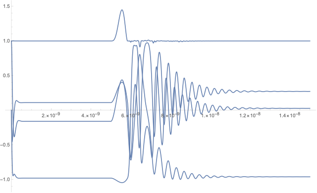
The peak at the delayed time t about 5.5 ns for the invariant is a violation of the foundational physics for the problem. Since the problem is reduced from the mathematical standpoint this is the solution.
The best path for a more physical solution will be to model that the peak does not appear. For example model some counter current from the other side of the electric system or some immanent current sources that delay in the calculated or near calculated manner.
Another interpretation might be, that there are times of unphysical solutions unavoidable in this modeling. Another one is a sign is set wrong. Nevertheless, the system recovers.
Remove["Global`*"] (*PARAMETERS*) γ = 1.76*10.^7*10.^4 (*T^-1s^-1*); α = 0.06; θsh = 0.3; Ms \ = 7.*10.^5;(*A/m*)tFM = 2.*10.^-9;(*m*)currAMP = 30.*10.^-3 (*A*); sHM = 10.*10.^-6*3.*10.^-9(*m^2,tHM=3 nm*); Hamp = 0.03; Hk = 0.1; a = 0. °; b = 0. °; c = 0. °; Ang = 0. °; temp = 3; rad = 20.*10.^-9;(*Thermal effect*)kTL = 2.; tSt = 0.; tFin = 1.5*10.0^-8; tStep = 1.*10.0^-12; (*CURRENT PULSE*) tPulse = 5.*10^-9; tRise = 0.5*10^-9; jcurr[t_] := Piecewise[{{1., -1 <= t <= tPulse}}, 0.]; Cjconst = (3.29375`*^-16) (θsh/Ms/tFM)*currAMP/sHM; Cj[t_] := Cj[t] = jcurr[t]*Cjconst; (*FIELD COMPONENTS*) σf[temp_, rad_] := Sqrt[(2.*α*1.38*10.^-23*temp)/(γ*Ms*tFM*3.1415*rad^2* tStep)]; σ = σf[temp, rad];(*stand.dev*) RandComp[] := RandomVariate[NormalDistribution[0., σ]]/ Sqrt[3.];(*random component*)Happ = ({{Cos[c], -Sin[c], 0.}, {Sin[c], Cos[c], 0.}, {0., 0., 1.}}).({{Cos[b], 0., Sin[b]}, {0., 1., 0.}, {-Sin[b], 0., Cos[b]}}).({{1., 0., 0.}, {0., Cos[a], -Sin[a]}, {0., Sin[a], Cos[a]}}).({{Hamp* Cos[Ang]}, {Hamp*(-Sin[ Ang])}, {0.}});(*permanent applied component*) Hrand[t_] := Hrand[t] = {RandComp[], RandComp[], RandComp[]}; H[t_, mz_] := Flatten[Happ + Hrand[t] + {0., -kTL*Cj[t], Hk*mz}] (*ODE SYSTEM*) t0 = 0; sol0 = NDSolve[({{mX'[ t] == γ (-mY[t]*H[t, mZ[t]][[3]] + mZ[t]*H[t, mZ[t]][[2]] - α (mY[ t] (mX[t]*H[t, mZ[t]][[2]] - mY[t]*H[t, mZ[t]][[1]]) - mZ[t] (mZ[t]*H[t, mZ[t]][[1]] - mX[t]*H[t, mZ[t]][[3]])) + Cj[t]*mY[t]*mX[t] + α*Cj[t]*mZ[t]), mX[0] == 0.}, {mY'[ t] == γ (-mZ[t]*H[t, mZ[t]][[1]] + mX[t]*H[t, mZ[t]][[3]] - α (mZ[ t] (mY[t]*H[t, mZ[t]][[3]] - mZ[t]*H[t, mZ[t]][[2]]) - mX[t] (mX[t]*H[t, mZ[t]][[2]] - mY[t]*H[t, mZ[t]][[1]])) - Cj[t] (mX[t]^2 + mZ[t]^2)), mY[0] == 0.}, {mZ'[ t] == γ (-mX[t]*H[t, mZ[t]][[2]] + mY[t]*H[t, mZ[t]][[1]] - α (mX[ t] (mZ[t]*H[t, mZ[t]][[1]] - mX[t]*H[t, mZ[t]][[3]]) - mY[t] (mY[t]*H[t, mZ[t]][[3]] - mZ[t]*H[t, mZ[t]][[2]])) + Cj[t]*mY[t]*mZ[t] - α*Cj[t]*mX[t]), mZ[0] == 1.}}), {mX, mY, mZ}, {t, tSt, tFin}, StartingStepSize -> 10.^-16, Method -> {"Projection", Method -> "Automatic", "Invariants" -> (mX[t]^2 + mY[t]^2 + mZ[t]^2 == 1)}, AccuracyGoal -> 15, PrecisionGoal -> 10000] StepDataPlot[sol0, PlotRange -> {tSt, tFin}] Plot[{mX[t], mY[t], mZ[t], mX[t]^2 + mY[t]^2 + mZ[t]^2} /. sol0, {t, tSt, tFin}] Great


