displayed rather than inline MathJax
Source Link
Michael Hardy
  • 13.1k
  • 2
  • 36
  • 62

I am trying to get a better understanding of kernel density estimation.

Using the definition from Wikipedia: https://en.wikipedia.org/wiki/Kernel_density_estimation#Definition

$ \hat{f_h}(x) = \frac{1}{n}\sum_{i=1}^n K_h (x - x_i) \quad = \frac{1}{nh} \sum_{i=1}^n K\Big(\frac{x-x_i}{h}\Big) $$$ \hat{f_h}(x) = \frac{1}{n}\sum_{i=1}^n K_h (x - x_i) \quad = \frac{1}{nh} \sum_{i=1}^n K\Big(\frac{x-x_i}{h}\Big) $$

Let's take $K()$ to be a rectangular function which gives $1$ if $x$ is between $-0.5$ and $0.5$ and $0$ otherwise, and $h$ (window size) to be 1.

I understand that the density is a convolution of two functions, but I am not sure I know how to define these two functions. One of them should (probably) be a function of the data which, for every point in R, tells us how many data points we have in that location (mostly $0$). And the other function should probably be some modification of the kernel function, combined with the window size. But I am not sure how to define it.

Any suggestions?

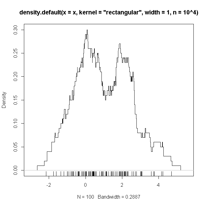
Bellow is an example R code which (I suspect) replicates the settings I defined above (with a mixture of two Gaussians and $n=100$), on which I hope to see a "proof" that the functions to be convoluted are as we suspect.

# example code: set.seed(2346639) x <- c(rnorm(50), rnorm(50,2)) plot(density(x, kernel='rectangular', width=1, n = 10**4)) rug(x) 
enter image description here

I am trying to get a better understanding of kernel density estimation.

Using the definition from Wikipedia: https://en.wikipedia.org/wiki/Kernel_density_estimation#Definition

$ \hat{f_h}(x) = \frac{1}{n}\sum_{i=1}^n K_h (x - x_i) \quad = \frac{1}{nh} \sum_{i=1}^n K\Big(\frac{x-x_i}{h}\Big) $

Let's take $K()$ to be a rectangular function which gives $1$ if $x$ is between $-0.5$ and $0.5$ and $0$ otherwise, and $h$ (window size) to be 1.

I understand that the density is a convolution of two functions, but I am not sure I know how to define these two functions. One of them should (probably) be a function of the data which, for every point in R, tells us how many data points we have in that location (mostly $0$). And the other function should probably be some modification of the kernel function, combined with the window size. But I am not sure how to define it.

Any suggestions?

Bellow is an example R code which (I suspect) replicates the settings I defined above (with a mixture of two Gaussians and $n=100$), on which I hope to see a "proof" that the functions to be convoluted are as we suspect.

# example code: set.seed(2346639) x <- c(rnorm(50), rnorm(50,2)) plot(density(x, kernel='rectangular', width=1, n = 10**4)) rug(x) 

enter image description here

I am trying to get a better understanding of kernel density estimation.

Using the definition from Wikipedia: https://en.wikipedia.org/wiki/Kernel_density_estimation#Definition

$$ \hat{f_h}(x) = \frac{1}{n}\sum_{i=1}^n K_h (x - x_i) \quad = \frac{1}{nh} \sum_{i=1}^n K\Big(\frac{x-x_i}{h}\Big) $$

Let's take $K()$ to be a rectangular function which gives $1$ if $x$ is between $-0.5$ and $0.5$ and $0$ otherwise, and $h$ (window size) to be 1.

I understand that the density is a convolution of two functions, but I am not sure I know how to define these two functions. One of them should (probably) be a function of the data which, for every point in R, tells us how many data points we have in that location (mostly $0$). And the other function should probably be some modification of the kernel function, combined with the window size. But I am not sure how to define it.

Any suggestions?

Bellow is an example R code which (I suspect) replicates the settings I defined above (with a mixture of two Gaussians and $n=100$), on which I hope to see a "proof" that the functions to be convoluted are as we suspect.

# example code: set.seed(2346639) x <- c(rnorm(50), rnorm(50,2)) plot(density(x, kernel='rectangular', width=1, n = 10**4)) rug(x) 

enter image description here

Notice removed Reward existing answer by Glen_b
Bounty Ended with whuber's answer chosen by Glen_b
Notice added Reward existing answer by Glen_b
Bounty Started worth 50 reputation by Glen_b
edited tags
Link
Danica
  • 25.5k
  • 2
  • 79
  • 142
Tweeted twitter.com/#!/StackStats/status/393128714831417344
small tweaks to presentation
Source Link
Nick Cox
  • 62.1k
  • 8
  • 145
  • 231

I am trying to get a better understanding of kernel density estimation.

Using the definition from Wikipedia: https://en.wikipedia.org/wiki/Kernel_density_estimation#Definition

$ \hat{f}_h(x) = \frac{1}{n}\sum_{i=1}^n K_h (x - x_i) \quad = \frac{1}{nh} \sum_{i=1}^n K\Big(\frac{x-x_i}{h}\Big) $$ \hat{f_h}(x) = \frac{1}{n}\sum_{i=1}^n K_h (x - x_i) \quad = \frac{1}{nh} \sum_{i=1}^n K\Big(\frac{x-x_i}{h}\Big) $

Let's take k$K()$ to be a rectangular function which gives 1$1$ if "x"$x$ is between -0.5 to 0.5$-0.5$ and (0$0.5$ and $0$ otherwise), and h $h$ (window size) to be 1.

I understand that the density is a convolution of two functions, but I am not sure I know how to define these two functions. One of them should (probably) be a function of the data which, for every point in R, tells us how many data points we have in that location (mostly 0$0$). And the other function should probably be some modification of the kernel function, combined with the window size. But I am not sure how to define it.

Any suggestions?

Bellow is an example R code which (I suspect) replicates the settings I defined above (with a mixture of two GaussianGaussians and n=100$n=100$), on which I hope to see a "proof" that the functions to be convoluted are as we suspect.

# example code: set.seed(2346639) x <- c(rnorm(50), rnorm(50,2)) plot(density(x, kernel='rectangular', width=1, n = 10**4)) rug(x) 

enter image description here

I am trying to get a better understanding of kernel density estimation.

Using the definition from Wikipedia: https://en.wikipedia.org/wiki/Kernel_density_estimation#Definition

$ \hat{f}_h(x) = \frac{1}{n}\sum_{i=1}^n K_h (x - x_i) \quad = \frac{1}{nh} \sum_{i=1}^n K\Big(\frac{x-x_i}{h}\Big) $

Let's take k to be a rectangular function which gives 1 if "x" is between -0.5 to 0.5 (0 otherwise), and h (window size) to be 1.

I understand that the density is a convolution of two functions, but I am not sure I know how to define these two functions. One of them should (probably) be a function of the data which, for every point in R, tells us how many data points we have in that location (mostly 0). And the other function should probably be some modification of the kernel function, combined with the window size. But I am not sure how to define it.

Any suggestions?

Bellow is an example R code which (I suspect) replicates the settings I defined above (with a mixture of two Gaussian and n=100), on which I hope to see a "proof" that the functions to be convoluted are as we suspect.

# example code: set.seed(2346639) x <- c(rnorm(50), rnorm(50,2)) plot(density(x, kernel='rectangular', width=1, n = 10**4)) rug(x) 

enter image description here

I am trying to get a better understanding of kernel density estimation.

Using the definition from Wikipedia: https://en.wikipedia.org/wiki/Kernel_density_estimation#Definition

$ \hat{f_h}(x) = \frac{1}{n}\sum_{i=1}^n K_h (x - x_i) \quad = \frac{1}{nh} \sum_{i=1}^n K\Big(\frac{x-x_i}{h}\Big) $

Let's take $K()$ to be a rectangular function which gives $1$ if $x$ is between $-0.5$ and $0.5$ and $0$ otherwise, and $h$ (window size) to be 1.

I understand that the density is a convolution of two functions, but I am not sure I know how to define these two functions. One of them should (probably) be a function of the data which, for every point in R, tells us how many data points we have in that location (mostly $0$). And the other function should probably be some modification of the kernel function, combined with the window size. But I am not sure how to define it.

Any suggestions?

Bellow is an example R code which (I suspect) replicates the settings I defined above (with a mixture of two Gaussians and $n=100$), on which I hope to see a "proof" that the functions to be convoluted are as we suspect.

# example code: set.seed(2346639) x <- c(rnorm(50), rnorm(50,2)) plot(density(x, kernel='rectangular', width=1, n = 10**4)) rug(x) 

enter image description here

Source Link
Tal Galili
  • 22.1k
  • 36
  • 150
  • 216
Loading