There's a nice discussion of this problem in Embedded Signal Processing with the Micro Signal Architecture, roughly between pages 63 and 69. On page 63, it includes a derivation of the exact recursive moving average filter (which niaren gave in his answerhis answer),
$$ H(z) = { 1 \over{N} } { 1 - z^{-N} \over { 1 - z^{-1} } }. $$
For convenience with respect to the following discussion, it corresponds to the following difference equation:
$$ y_n = y_{n-1} + {1\over{N} }(x_n - x_{n-N}). $$
The approximation which puts the filter into the form you specified requires assuming that $x_{n-N} \approx y_{n-1}$, because (and I quote from pg. 68) "$y_{n-1}$ is the average of $x_n$ samples". That approximation allows us to simplify the preceding difference equation as follows:
$$ \begin{array}\\ y_{n} = y_{n-1} + {1\over{N}}(x_n - y_{n-1}) \\ y_{n} = y_{n-1} - {1\over{N}} y_{n-1} + {1\over{N}}x_n \\ y_{n} = (1-{1\over{N}})y_{n-1} + {1\over{N}}x_n. \end{array} $$
Setting $\alpha = {1\over{N}}$, we arrive at your original form, $y_{n} = \alpha x_n + (1-\alpha)y_{n-1}$, which shows that the coefficient you want (with respect to this approximation) is exactly $1\over{N}$ (where $N$ is the number of samples).
Is this approximation the "best" in some respect? It's certainly elegant. Here's how the magnitude response compares [at 44.1kHz] for N = 3, and as N increases to 10 (approximation in blue):
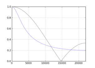
![N=[3,10]](https://i.sstatic.net/qOpek.png)
As Peter's answerPeter's answer suggests, approximating an FIR filter with a recursive filter can be problematic under a least squares norm. An extensive discussion of how to solve this problem in general can be found in JOS's thesis, Techniques for Digital Filter Design and System Identification with Application to the Violin. He advocates the use of the Hankel Norm, but in cases where the phase response doesn't matter, he also covers Kopec's Method, which might work well in this case (and uses an $L^2$ norm). A broad overview of the techniques in the thesis can be found here. They may yield other interesting approximations.