close all;clear all;clc % MATLAB script available by email [email protected]
1.- Simulating 2 random phases
ph1_deg=.1*(2*(randi([1 2],1,1)-1.5))*randi([150 1800],1,1) ph2_deg=.1*(2*(randi([1 2],1,1)-1.5))*randi([150 1800],1,1) ph1=ph1_deg*pi/180 ph2=ph2_deg*pi/180 dph=abs(ph1-ph2) dph_deg=dph*180/pi
2.- Generating signals
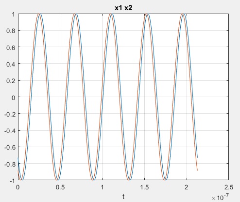
same carrier 2 random different phases within [15 180]deg
f1=23.5e6 % [Hz] T1=1/f1 fs=100*f1; dt=1/fs; amount_cycles_measured=5 t=[0:dt:amount_cycles_measured*T1]; x1=sin(2*pi*f1*t+ph1); x2=sin(2*pi*f1*t+ph2); figure(1) plot(t,x1,t,x2) grid on xlabel('t') title('x1 x2')

3.- So far so good, one checks a trigonometry manual and there you have it : Multiply both carriers and the phase difference should readily come up.
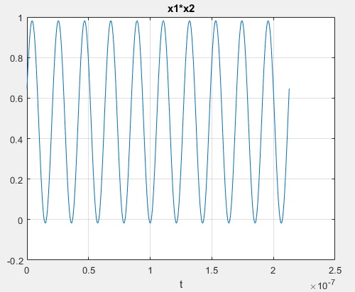
But the resulting theoretical expression is supposed to be time independent, it's supposed to be DC.
In RF boards DC is almost always blocked preventing access into different RF stages.
Shure Xilinx boards have some DC protection to prevent DC hitting signal processing modules.
x12=x1.*x2; figure(2) plot(t,(x12)) grid on xlabel('t') title('x1*x2')

wasn't this supposed to be a clear measurement of the phase difference?
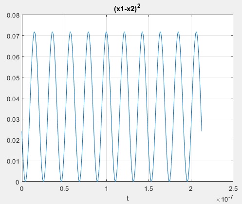
perhaps the power of the difference
figure(3) plot(t,(x1-x2).^2) grid on xlabel('t') title('(x1-x2)^2')

4.- There's a clear loss of amplitude accuracy, the amplitude that has to supply the DC reading for the phase difference.
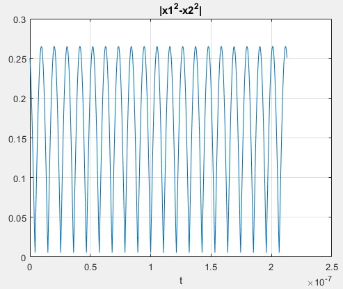
May be another difference of powers?
x3=x1.^2; x4=x2.^2; x34=abs(x3-x4); figure(4) plot(t,x34) grid on xlabel('t') title('|x1^2-x2^2|')

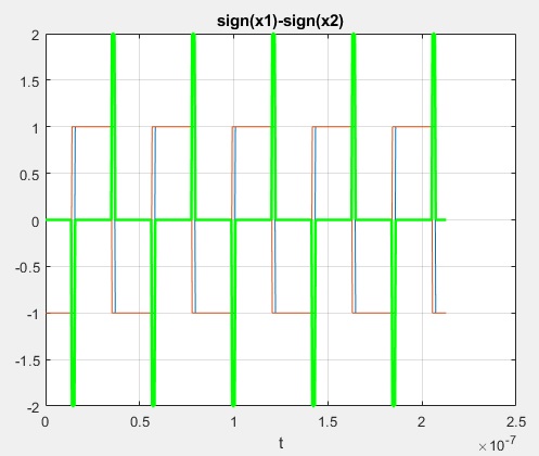
5.- Let's focus on the zero crossings
x5=sign(x1); x6=sign(x2); x56=x5-x6; figure(5) plot(t,x5,t,x6) hold on plot(t,x56,'g','LineWidth',2) grid on xlabel('t') title('sign(x1)-sign(x2)')

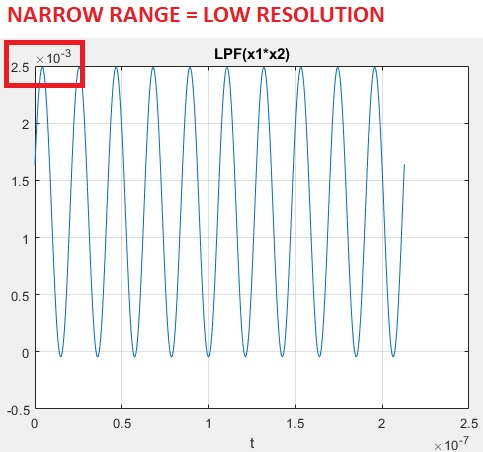
6.- Perhpaps Low Pass Filtering x1.*x2 increases DC accuracy?
sr = dsp.SignalSource; sr.Signal = x12; sink = dsp.SignalSink; nth=20 % filter order wsn=.25 % normalized Nyquist freq = fs/2 fir = dsp.FIRFilter(fir1(nth,wsn)); % .25 fraction of Nyquist freq sa = dsp.SpectrumAnalyzer('SampleRate',fs,... 'PlotAsTwoSidedSpectrum',false,... 'OverlapPercent', 80, 'PowerUnits','dBW',... 'YLimits', [-150 -10]); while ~isDone(sr) input = sr(); filteredOutput = fir(input); sink(filteredOutput); end filteredResult = sink.Buffer; % fvtool(fir,'Fs',f1/2) figure(6) plot(t,filteredResult) grid on xlabel('t') title('LPF(x1*x2)')

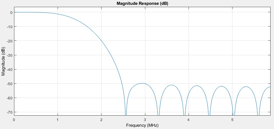
filter used 
Low Pass Filtered signal containing the phase difference does not show the expected accuracy to measure phase differences.
And this is without noise.
Observe that the peak value is 2.5e-3 .
To measure with precision a phase difference it is convenient to work with for instance a [0 5]V range, not with mV if possible.
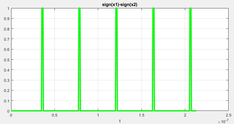
7.- Squaring input signals
x56(x56<0)=0; x56=.5*x56; figure(7) plot(t,x56) hold on plot(t,x56,'g','LineWidth',3) grid on xlabel('t') title('sign(x1)-sign(x2)')

All that's left is to measure pulse widths, perhaps average a few of them and translate pulsewidth (time) to phase (difference)
Do not demodulate to DC.
All you need are the difference between squared input signals
d1_deg=360*numel(x56(x56==0))/numel(x56) if d1_deg>180 d1_deg=360-d1_deg; end
comparing
d1_deg = 14.371257485029957 dph_deg = 15.099999999999991
d1_deg is measured phase difference and dph_deg is expected value.
absolute error
err_abs=abs(d1_deg-dph_deg) = 0.728742514970033
relative error
err_rel=err_abs/dph_deg*100 = 4.826109370662475
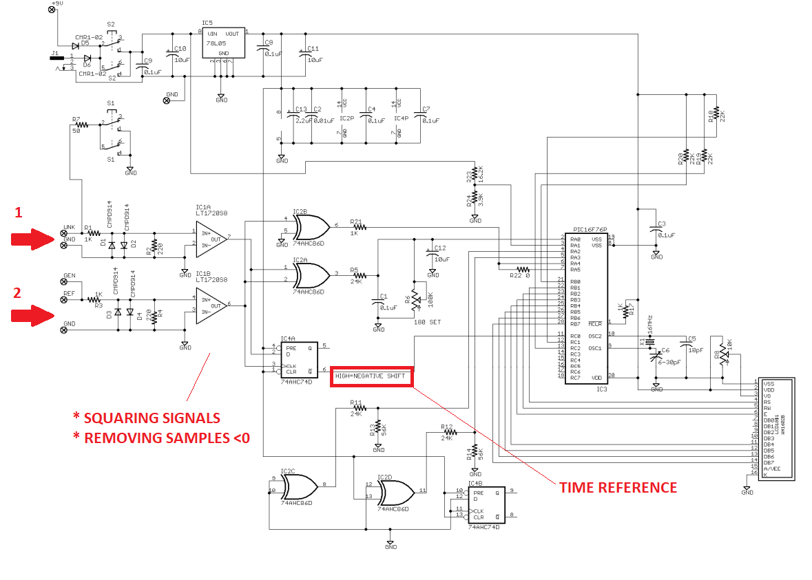
8.- Example MFJ222 phase difference meter [1 50] MHz Manufactured by MFJ Enterprises, 300 Industrial Park Road, Starkville, MS 39759. Phone: (662) 323-5869
MFJ schematic (public, available online) showing signals conditioning

The sign ambiguity is not relevant because one may assume that dph=ph2-ph1 in a certain order, but if the phase difference exceeds 180deg there's again a sign shift in the phase difference.
Therefore the important measurement is the absolute difference between phases.
In the measurement procedure one has to choose what signal is the reference and what signal phase is measured against the eference, thus deciding the order to consider for the difference,
9.- There's room for accuracy improvement
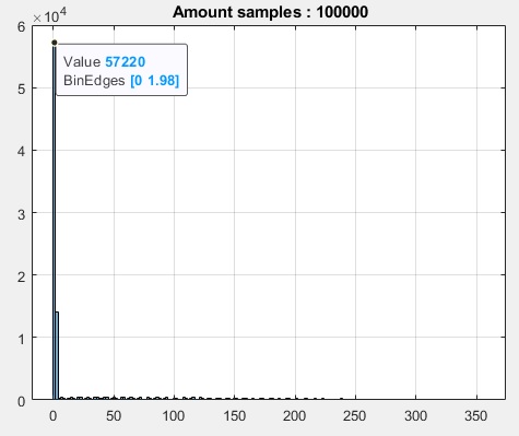
Measuring accuracy repeating for 1e5 rounds
log_err_abs=[]; log_err_rel=[]; num_samples=100000 for k=1:1:num_samples ph1_deg=.1*(2*(randi([1 2],1,1)-1.5))*randi([150 1800],1,1); ph2_deg=.1*(2*(randi([1 2],1,1)-1.5))*randi([150 1800],1,1); ph1=ph1_deg*pi/180; ph2=ph2_deg*pi/180; dph=abs(ph1-ph2); dph_deg=dph*180/pi; x1=sin(2*pi*f1*t+ph1); x2=sin(2*pi*f1*t+ph2); x12=x1.*x2; x5=sign(x1); x6=sign(x2); x56=x5-x6; x56(x56<0)=0; x56=.5*x56; d1_deg=360*numel(x56(x56==0))/numel(x56); if d1_deg>180 d1_deg=360-d1_deg; end % dph_deg; % comparing err_abs=abs(d1_deg-dph_deg); % absolute error err_rel=err_abs/dph_deg*100; % relative error log_err_abs=[log_err_abs err_abs]; log_err_rel=[log_err_rel err_rel]; end figure(8) histogram(log_err_abs,180) grid on title([' Amount samples : ' num2str(num_samples)])

The few scattered large errors are sign inversions that are not considered in the line with clause if d1_deg>360 ..
10.- Regarding amplitude/phase noise, as long as 'small' the floating configuration show in the MFJ222 schematic is a the correct approach for the noise on both branches cancel each other, that never happens, such is the nature of noise, but it get's reduced, it's common practice in RF circuits.
Thanks for reading this answer.
If this answer is found useful would you please conside clicking on the accepted answer.

