0
\$\begingroup\$

I am trying to replicate a result from a textbook that I am using to study input filter design for buck converters. enter image description here

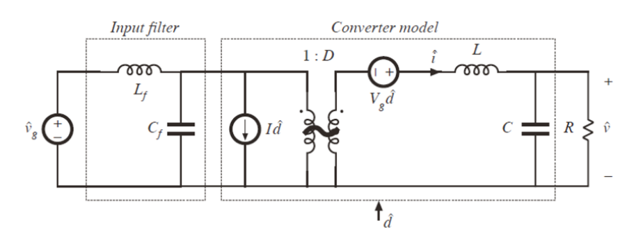
The parameters for the converter and filter are as follows:

  • D = 0.5
  • L = 100 μH
  • C = 100 μF
  • R = 3 Ω
  • Lf = 330 μH
  • Cf = 470 μF

The Bode plot in the textbook is shown below. enter image description here

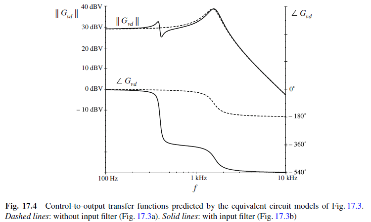
I used MATLAB to create a similar Bode response, using this code:

opts = bodeoptions; opts.FreqUnits = 'Hz'; vd=5; R=3; D=0.5; vo_desired=D*vd; L=100e-6; C=100e-6; L_f=330e-6; C_f=470e-6; Gd0=vd; w0=1/sqrt(L*C); Q=R*sqrt(C/L); Gvd=tf(Gd0,[1/(w0)^2,1/(Q*w0),1]); Z=tf([L_f,0],[L_f*C_f,0,1]); ZN=tf(-R/D^2,1); ZD=tf([R*C*L,L,R],[C*R,1])/D^2; Gvd_new=Gvd*((1+Z/ZN)/(1+Z/ZD)); bode(Gvd,opts,'r--') hold on; dcm = datacursormode; dcm.Enable = 'on'; grid bode(Gvd_new,opts) legend('G_{vd}','G_{vd,new}') 

This results in this Bode: enter image description here

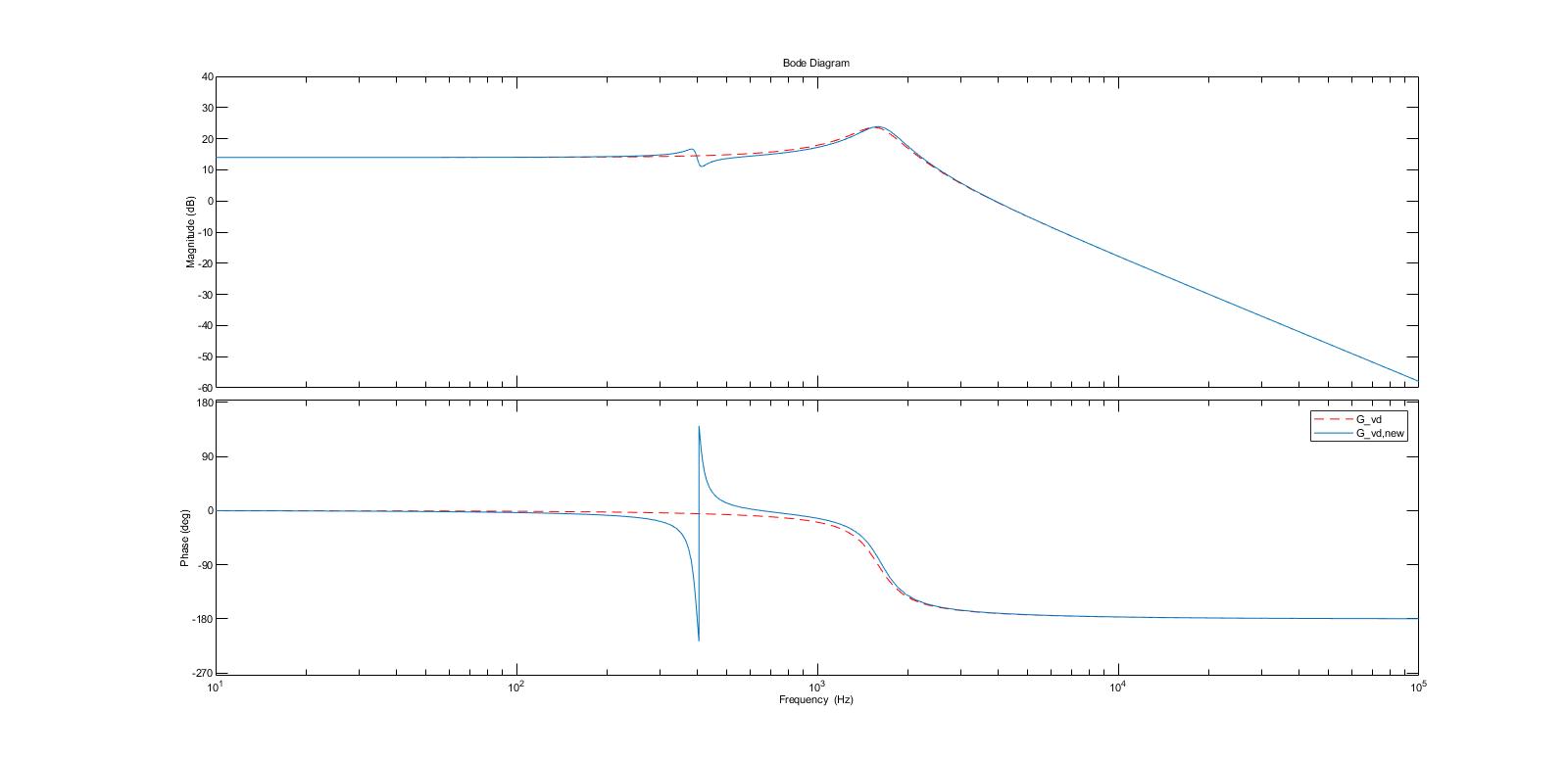
As you can see from the attached Bode plot I generated, the magnitude response seems to match what is shown in the textbook, but the phase response is significantly different. Am I missing something in my code or calculation?

\$\endgroup\$
5
  • \$\begingroup\$ A schematic of what the book plot represents is missing and, what your code represents has no schematic. \$\endgroup\$ Commented Feb 7, 2023 at 11:16
  • \$\begingroup\$ The only obvious, big difference between the phase plots is phase unwrapping. The textbook "unwrapped" the phase, your Matlab plot didn't. \$\endgroup\$ Commented Feb 7, 2023 at 11:46
  • \$\begingroup\$ @Andyaka apologies, the plots are for regular buck converters with an LC filter, I added the schematic. \$\endgroup\$ Commented Feb 7, 2023 at 11:47
  • \$\begingroup\$ @JRE can you elaborate more please? what do you mean by unwrapping? \$\endgroup\$ Commented Feb 7, 2023 at 11:50
  • 2
    \$\begingroup\$ The phase of the signal goes outside of -180 and 180 degrees in the textbook example. It ranges from 0 degrees to 540 degrees. Your example forces the phase to stay between -180 and 180 degrees. There's a discontinuity in you plot where the phase goes above 180 degrees and "wraps around" to -180 degrees. "Phase unwrapping" is used to make the phase continuous. Here's how you apply it in MATLAB. \$\endgroup\$ Commented Feb 7, 2023 at 11:55

1 Answer 1

1
\$\begingroup\$

The general shape of your plot appears to match that of the textbook plot.

The biggest difference that I see is that the plot you made with MATLAB has a phase wrap-around while the textbook plot has the phase "unwrapped."

The MATLAB plot is constrained to stay between -180 and 180 degrees. That causes a discontinuity where the phase would exceed 180 degrees.

The textbook plot is continuous. It ranges from 0 to 540 degrees.

Your MATLAB program probably has "PhaseWrapping = 'on'" set in the "bodeoptions" somewhere. Since the default is "PhaseWrapping = 'off'", it must be your code that is turning it on.

\$\endgroup\$
1
  • \$\begingroup\$ Thank you so much, this might be an issue in the matlab version I am using, because i didn't anywhere in my code set the phase wrapping on. But that's ok fine, I just wanted to make sure I didn't make a mistake somewhere. Thanks again \$\endgroup\$ Commented Feb 8, 2023 at 9:02

Start asking to get answers

Find the answer to your question by asking.

Ask question

Explore related questions

See similar questions with these tags.