Named functions are user-created, reusable formulas within a Google Sheet. You can use them across all sheets in the same workbook where they are saved. To use a named function in a different spreadsheet, you can either recreate it manually or import it from a workbook where it already exists.

Named functions behave like built-in formulas: as you type the function name, Google Sheets shows it in the formula list and provides formula help. The efficiency of the function depends on the formula you define.

Custom Named Functions vs. Unnamed Functions

When we talk about custom named functions, it’s useful to contrast them with unnamed functions:

• Named functions: Created through the Google Sheets menu with placeholder arguments, reusable anywhere in the workbook.
• Unnamed functions: Functions without a name, created using the LAMBDA function.

Example of a Named Function

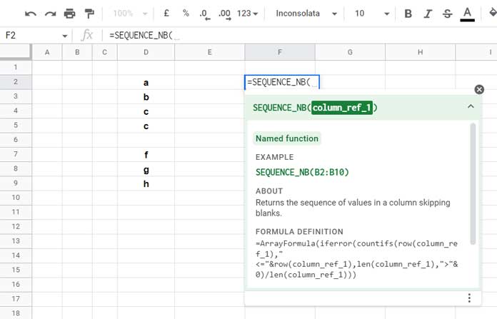
SEQUENCE_NB(column_ref_1) is a named function that returns sequence numbers corresponding to non-empty cells in another column. We will create this function later in the tutorial.

=SEQUENCE_NB(D2:D)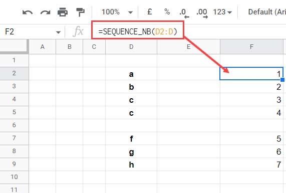

Place this in row 2 of any empty column (e.g., F2) to get sequence numbers corresponding to non-blank cells in column D.

You can reuse it across the workbook like any built-in function:

=SEQUENCE_NB(A2:A) =SEQUENCE_NB(Sheet2!I:I)

Equivalent Unnamed Function

The same logic can be implemented with a LAMBDA function:

=LAMBDA(column_ref_1, ArrayFormula(IF(LEN(column_ref_1), COUNTIFS(ROW(column_ref_1), "<="&ROW(column_ref_1), LEN(column_ref_1), ">0"), "")))(D2:D)

Or directly as a formula:

=ArrayFormula(IF(LEN(D2:D), COUNTIFS(ROW(D2:D), "<="&ROW(D2:D), LEN(D2:D), ">0"), ""))

Key Difference:

• Unnamed function: Created using the LAMBDA function, these are often used as helper functions with BYROW, BYCOL, SCAN, REDUCE, MAP, or MAKEARRAY. Placeholders like column_ref_1 are defined within the LAMBDA itself.
• Named function: Placeholders are defined using the Named Functions menu, making reuse easier without typing the full formula.

When to Consider Creating a Named Function

Named functions are especially useful when:

• You need to reuse complex formulas multiple times in a sheet or workbook.
• You want to simplify formulas for team members or collaborators.
• You need to standardize calculations across multiple sheets or reports.

How Named Functions Differ in Excel and Google Sheets

Excel: You first convert a formula to a LAMBDA function, then define it in Name Manager.

Google Sheets: You don’t need to write a LAMBDA first.

• Copy your working formula.
• Go to Data > Named functions.
• Replace cell/range references with meaningful placeholders (text) for inputs.

Example: Replace A2:A with column_reference.

How to Create a Named Function in Google Sheets

We’ll create two examples to demonstrate how to convert formulas into named functions: SEQUENCE_NB (one argument) and FLIP_DATA (two arguments).

Example 1: SEQUENCE_NB (One Argument)

This function returns sequential numbers corresponding to non-empty cells in a column.

Formula:

=ArrayFormula(IF(LEN(D2:D), COUNTIFS(ROW(D2:D), "<="&ROW(D2:D), LEN(D2:D), ">0"), ""))

Creating the named function:

1. Copy the formula.
2. Go to Data > Named functions > Add new function.
3. Name the function: SEQUENCE_NB. Avoid:
   • Built-in function names
   • TRUE/FALSE
   • A1 or R1C1 references
   • Spaces or special characters (except underscore)
   • Names starting with a number
   • Overly long names (>255 characters)
4. Add a description: “Returns the sequence of values in a column skipping blanks.”
5. Add the argument placeholder: column_ref_1 (don’t forget to click the ↵ Enter icon).
6. Paste the formula and replace D2:D with the placeholder:

=ArrayFormula(IF(LEN(column_ref_1), COUNTIFS(ROW(column_ref_1), "<="&ROW(column_ref_1), LEN(column_ref_1), ">0"), ""))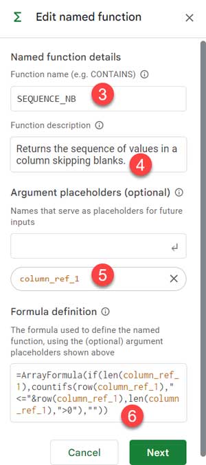

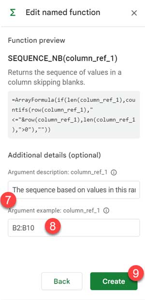
7. Click Next, fill in the argument description and example reference (e.g., B2:B10), then click Create.

You can now reuse SEQUENCE_NB anywhere in the workbook, just like a built-in function:

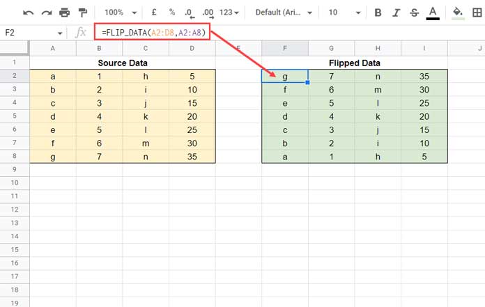
=SEQUENCE_NB(A2:A) =SEQUENCE_NB(Sheet2!I:I)

Example 2: FLIP_DATA (Two Arguments)

This function flips a data range vertically.

Formula:

=SORT(A2:C5, ROW(A2:A5)*N(A2:A5<>""), 0)

Creating the named function:

The process is the same as in Example 1. Key differences:

• Function name: FLIP_DATA
• Description: “Given a range, returns a vertically flipped data range.”
• Argument placeholders:
  • flip_range → the range to flip
  • first_col_range → the first column used for sorting
• Copy and paste the formula, then replace the cell references in the formula with placeholders:

=SORT(flip_range, ROW(first_col_range)*N(first_col_range<>""), 0)

• Click Next and optionally enter example values: A2:C5 for flip_range and A2:A5 for first_col_range.

Click Create, and the named function is ready to use across the workbook.

How to Delete or Modify Named Functions

1. Go to Data > Named functions.
2. Click the three dots next to a function.
3. Choose Edit or Remove.

Note: You cannot delete multiple named functions at once.

Importing Named Functions from Another Workbook

1. Create all required named functions in a source sheet.
2. Open the destination Google Sheet.
3. Go to Data > Named functions > Import function.
4. Select the file containing your named functions.
5. Click Import All or select specific functions to import.

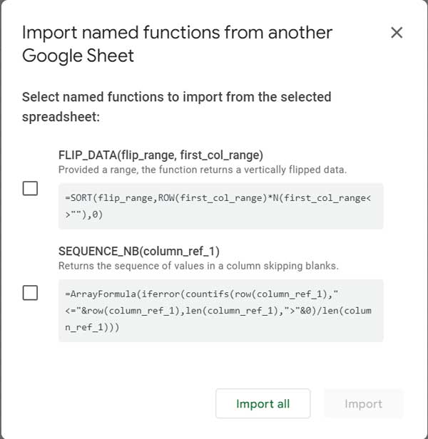
Now the imported named functions are available for use within this destination workbook.

Get My Ready-Made Named Functions in Google Sheets

• PUNCH_IN_OUT_SAME_ROW → Copy Punch Out Time to Punch In Row
• COPY_TO_MASTER_SHEET → Combine data across multiple tabs
• MERGE_TABLE_REMOVE_DUPLICATES → Remove duplicates by key column
• COMPARE_ALL_COLUMNS → Compare all columns for duplicates
• NEXT_RENEWAL_DATE → Next renewal date (monthly/yearly)
• AGE_CALC → Calculate age or duration
• REPT_ROWS → Repeat rows by varying N
• GANTT_CHART → Create Gantt charts easily
• LIST_ALL_DATES → Populate dates between two or more given dates
• AT_EACH_CHANGE → Aggregate results at value change rows
• CUSUM_BY_GROUP → Running total by group
• SPARKLINE_NEGATIVE_BAR → Sparkline for positive/negative values
• REF_SHEET_TABS → Reference a list of tab names in QUERY
• _3D → Creates 3D references
• SPLIT_EXPENSES → Split group expenses
• NUM_TO_WORDS_IND & NUM_TO_WORDS_US → Convert numbers to words
• CUSTOMTIMESLOTS → Create custom time slot sequences
• TOSENTENCECASE → Convert text to sentence case
• FLIP → Reverse order of rows or columns

Conclusion

Creating named functions in Google Sheets streamlines your workflow, reduces errors, and allows complex formulas to be reused easily across your workbook. With a few steps, you can turn any formula into a reusable tool, import it across workbooks, and simplify data management tasks.