")
")
 Converter Template for Google Sheets")
")


")
")


 in Excel & Google Sheets")


The REDUCE function in Google Sheets processes an array into a single accumulated result by repeatedly applying the same LAMBDA function to each element.
Many of you might have come across REDUCE in complex formulas—whether it’s merging data from multiple tabs or sheets, filtering, stacking arrays, and so on. In such cases, REDUCE doesn’t just return a single value. Instead, it returns an array by stacking the accumulated value at each iteration, either vertically or horizontally.
Understanding this behavior is just as important.
REDUCE Function Syntax and Arguments in Google Sheets
REDUCE syntax:
REDUCE(initial_value, array_or_range, LAMBDA)Where:
- initial_value – Sets the initial or starting value of the accumulator.
- array_or_range – The array or range to be reduced.
- LAMBDA – A custom LAMBDA function applied to each element of the array_or_range. It takes two arguments.
LAMBDA syntax:
LAMBDA(name1, name2, formula_expression)Here, name1 is the accumulator, and name2 represents the current element from the array. The formula expression performs the desired operation using these two.
To better understand the syntax of the REDUCE function in Google Sheets, try the example below.
How to Use the REDUCE Function in Google Sheets
Let’s try the following formula in an empty cell:
=REDUCE(0, {5; 4; 9; 10}, LAMBDA(a, v, a + v))This returns 28.
Here’s what’s happening:
- The initial value in the accumulator is
0. - The array to reduce is
{5; 4; 9; 10}. - We’ve defined two names:
afor the accumulator andvfor the current array element. - The formula expression is
a + v, which means that in each iteration, the current element is added to the accumulator.
So, it works like:(((0 + 5) + 4) + 9) + 10 = 28
The SCAN Connection
Now look at the SCAN function with a similar structure (just replace REDUCE with SCAN):
=SCAN(0, {5; 4; 9; 10}, LAMBDA(a, v, a + v))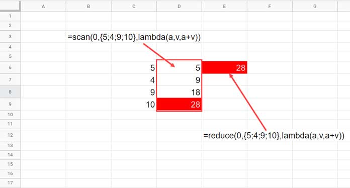
SCAN and REDUCE Functions – Similarities
While REDUCE returns only the final accumulated value, SCAN returns all intermediate values from each iteration.
Stacking in REDUCE
Now replace a + v in the REDUCE formula with VSTACK(a, CHOOSEROWS(a, -1) + v), like this:
=REDUCE(0, {5; 4; 9; 10}, LAMBDA(a, v, VSTACK(a, CHOOSEROWS(a, -1) + v)))Here, we start with an initial value of {0} and use VSTACK to keep adding each new sum to the growing array. CHOOSEROWS(a, -1) fetches the last value in the accumulator, and v is the current element in the array.
The result is a stacked (vertical) list of cumulative sums — similar to what the SCAN function returns — but it includes the initial value 0.
0
5
9
18
28
This is just a simple example to help you understand the concept. This technique is used in various advanced scenarios.
Examples of Using the REDUCE Function in Google Sheets
Below are four practical examples of using the REDUCE function in Google Sheets. Most of them can be replaced with regular formulas. But the purpose of these examples is to help you get familiar with how REDUCE works.
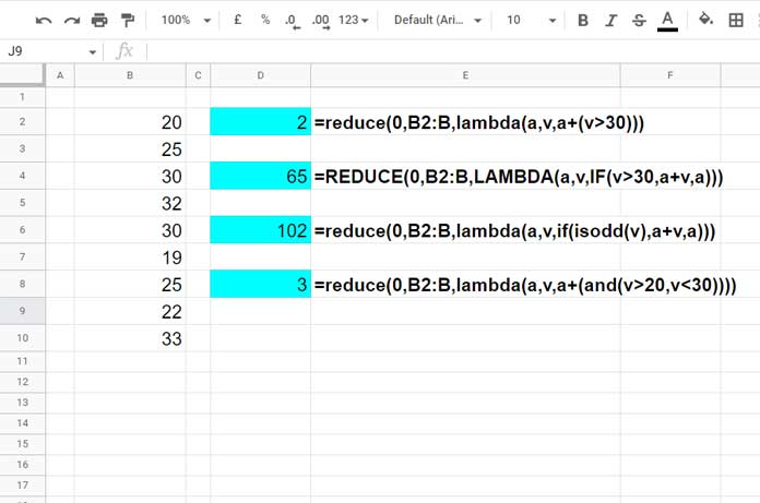
In all these examples, the initial value of the accumulator is 0.
If you set it to 100, the outputs in the cyan-highlighted cells would be 102, 165, 202, and 103 respectively.
1. REDUCE Function for Conditional Sum
The formulas in cells D4 and D6 show how to use the REDUCE function for conditional summing.
Formula in D4 – Sum if Value Is Greater Than 30
=REDUCE(0, B2:B, LAMBDA(a, v, IF(v > 30, a + v, a)))Equivalent to:
=SUMIF(B2:B, ">30")This adds only values greater than 30 to the accumulator.
Formula in D6 – Sum of Odd Numbers
=REDUCE(0, B2:B, LAMBDA(a, v, IF(ISODD(v), a + v, a)))SUMIF alternative:
=ARRAYFORMULA(SUMIF(ISODD(B2:B), TRUE, B2:B))These are great examples of using the REDUCE function in Google Sheets for condition-based summing.
2. REDUCE Function for Conditional Count
The formulas in D2 and D8 act as conditional counts.
Assume the values in B2:B represent the age of participants in a competition.
Formula in D2 – Count if Age Is Greater Than 30
=REDUCE(0, B2:B, LAMBDA(a, v, a + (v > 30)))Equivalent COUNTIF:
=COUNTIF(B2:B, ">30")Formula in D8 – Count if Age Is Between 20 and 30
=REDUCE(0, B2:B, LAMBDA(a, v, a + (AND(v > 20, v < 30))))Equivalent COUNTIFS:
=COUNTIFS(B2:B, ">20", B2:B, "<30")Other Miscellaneous Use Cases
Looking at the above examples, you might think the REDUCE function is mainly for conditional sums and counts.
But that’s not the case!
The REDUCE function in Google Sheets can do a lot more.
Example – Get the Last Numeric Value in Column B
=REDUCE(0, B:B, LAMBDA(a, v, IF(v = "", v + a, v)))To get the last numeric value in row 2, replace B:B with 2:2.
If the values are mixed (text + numbers), replace the initial value 0 with "", and use v & a instead of v + a.
Example – Conditional Total Using OFFSET
=REDUCE(0, A:A, LAMBDA(a, v, IF(v = "apple", OFFSET(v, 0, 1) + a, a)))This totals values in column B where the corresponding value in column A is “apple”.


