expression = (a b A Exp[-b (x - a)])/(a Exp[-b (x - a)] + 1)^2 + c Tan[x]
$$ \frac{a A b e^{-b (x-a)}}{\left(a e^{-b (x-a)}+1\right)^2}+c \tan (x) $$
Outline :
1) Removing c from the parameters
2) Finding some analytical solutions using FindInstance
3) Using Manipulate and ContourPlot to find roots in an equation with many parameters
4) Extracting the points from a given contour plot
5) Polishing results with better accuracy
1) Removing c from the parameters
For non zero c, we can absorb the dependence on c by dividing by c and using A->c*w :
expression2 = expression/c /. A -> w*c // Simplify
$$\frac{a b w e^{b (x-a)}}{\left(e^{b (x-a)}+a\right)^2}+\tan (x)$$
That way there is one less parameter to consider but do not forget to check separately the case c=0. In the following I will focus on c non zero.
2) Finding some analytical solutions using FindInstance
For generic parameters Mathematica can not find a root for expression above. However, it can find instances of roots using FindInstance. For example, if we consider a to be positive then :
FindInstance[{expression2 == 0, a > 0}, {x, a, b, w}]
{{x->9392403/3312026,a->26566113/18118801,b->30971405/14149612,w->-((256374004055212 (26566113/18118801+E^(2545583876943569930325/849117367154967579512))^2 Tan[9392403/3312026])/(822789844998765 E^(2545583876943569930325/849117367154967579512)))}}
If you want a symbolic solution regardless of whether the solution is in terms of the variable x or one of the parameters, consider Solve or Reduce.
3) Using Manipulate and ContourPlot to find roots in an equation with many parameters
We can visualize dependence on parameters using (recall that c=0 should be considered separately):
Note: I chose the ranges of parameters in an arbitrary manner
With[{expression2 = expression2}, Manipulate[ ContourPlot[expression2 == 0, {x, -4, 4}, {b, -4, 4}], {a, -4, 4}, {w, -4, 4}]]
4) Extracting the points from a given contour plot
If you want to extract the lines from a given value of a and w you can right click the plot and copy it and then paste into a new cell and use :
template of code below : points = Cases[Normal[... plot here ...], Line[x_] :> x, All]
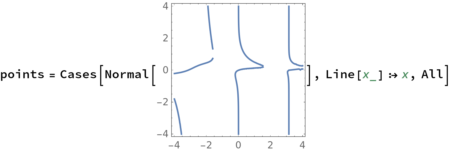
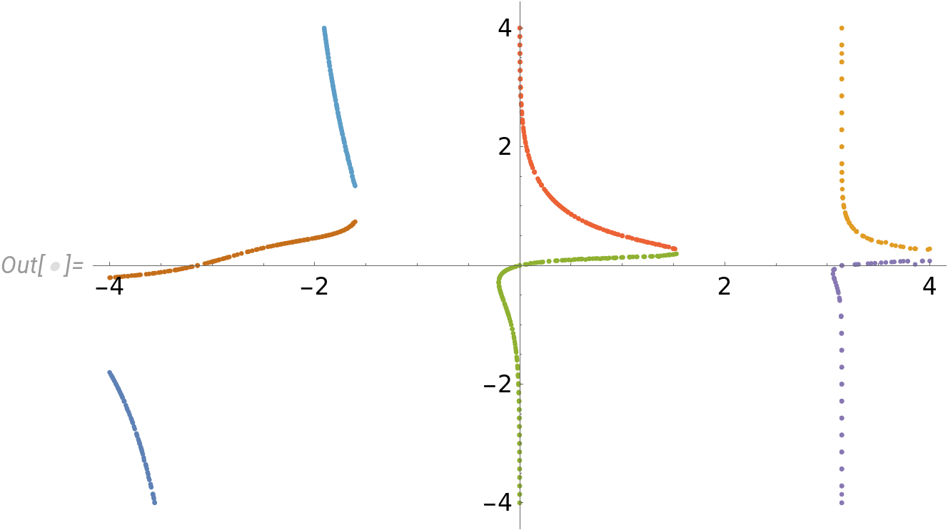
The points:
points // ListPlot
5) Polishing results with better accuracy
The points above might not be very accurate. In that case consider the numerical methods here: How to find seed values for solving nonlinear equations?
