Just for fun you can fit a 2nd order curve to the data around the peak and interpolate the actual peak. You have from your code, with a small mod to make sure we grab the first peak only:
data21 = Flatten[Abs[Fourier[Data1]]]; pos = Position[data21, Max[data21[[1 ;; Floor[Length[data21]/2]]]]][[1, 1]]; gf = (pos - 1)/((TimeEnd - TimeStart)) Now grab the points near the peak and do a 2nd order fit there
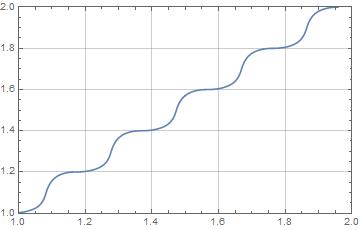
dr = Range[pos - 1, pos + 1] subdat = Transpose[{dr, data21[[dr]]}] posApprox = Solve[D[Fit[subdat, {1, x, x^2}, x], x] == 0] // Values // Flatten // First; gff = (posApprox - 1)/((TimeEnd - TimeStart)) Plot a comparison as you vary fB, between gff and fB. Not hideously shabby. Could probably find a better fitting function for the peak.
res = Table[{fB, TimeStart = 0; TimeEnd = 5; Data1 = Table[Sin[2 Pi fB x], {x, 0, 5, 1/10}]; sra = 10./1; inco = sra/Length[Data1]; fresa = Table[f, {f, 0, sra - inco, inco}]; data21 = Flatten[Abs[Fourier[Data1]]]; pos = Position[data21, Max[data21[[1 ;; Floor[Length[data21]/2]]]]][[1, 1]]; dr = Range[pos - 1, pos + 1]; subdat = Transpose[{dr, data21[[dr]]}]; posApprox = Solve[D[Fit[subdat, {1, x, x^2}, x], x] == 0] // Values // Flatten // First; gff = (posApprox - 1)/((TimeEnd - TimeStart))} , {fB, 1, 2, .01}]