Update 4. But we can reproduce solution from Update 2 using small modification to relaxation code
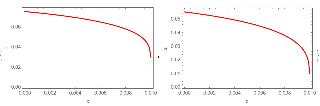
(*Two Coupled ODE Setup*)Clear["Global`*"] Needs["VariationalMethods`"] c = 1000; g = 3; m = c Exp[-g u[x]]; f = 1 - m z[x]^(d + 1); L = Sqrt[-f u'[x]^2 + 2 u'[x] z'[x] + 1]/z[x]^d; eq1 = EulerEquations[L, u[x], x]; eq2 = EulerEquations[L, z[x], x]; s = Solve[{eq1, eq2} /. d -> 3, {u''[x], z''[x]}][[1]] // Simplify; eq01 = (u''[x] - s[[1, 2]]); eq02 = (z''[x] - s[[2, 2]]); (*Parameters*) n = 100; h = (b - a)/(n - 1); a = 0; b = 10^-2; zf = 10^-2; uf = 0.03; {ui, zi} = {0.03319144803568739`, 0.013191393525749648`}; up = Sqrt[ Sqrt[((d - 1)^2/(1 - (d - 1)^2 (1 - c Exp[-g u[1]] (z[1])^(d + 1))))^2]] /. d -> 3; zp = -(1 - c Exp[-g u[1]] (z[1])^(d + 1)) Sqrt[ Sqrt[((d - 1)^2/(1 - (d - 1)^2 (1 - c Exp[-g u[1]] (z[1])^(d + 1))))^2]] /. d -> 3; (*Sparse Matrix Setup*) rule = {u''[x] -> ((u[i + 1] - 2 u[i] + u[i - 1])/h^2), u'[x] -> ((u[i + 1] - u[i - 1])/(2 h)), u[x] -> u[i], z''[x] -> ((z[i + 1] - 2 z[i] + z[i - 1])/h^2), z'[x] -> ((z[i + 1] - z[i - 1])/(2 h)), z[x] -> z[i]}; resid1 = h^2 eq01 /. rule; resid2 = h^2 eq02 /. rule; residbound1 = ((-3 u[1] + 4 u[2] - u[3]) - Sqrt[(2 up h)^2]); residbound2 = ((-3 z[1] + 4 z[2] - z[3]) - Sqrt[(2 zp h)^2]); parresid1 = {D[resid1, u[i - 1]], D[resid1, z[i - 1]], D[resid1, u[i]], D[resid1, z[i]], D[resid1, u[i + 1]], D[resid1, z[i + 1]]}; parresid2 = {D[resid2, u[i - 1]], D[resid2, z[i - 1]], D[resid2, u[i]], D[resid2, z[i]], D[resid2, u[i + 1]], D[resid2, z[i + 1]]}; parresidbound1 = D[residbound1, {{u[1], z[1], u[2], z[2], u[3], z[3]}}]; parresidbound2 = D[residbound2, {{u[1], z[1], u[2], z[2], u[3], z[3]}}]; mat = {parresid1, parresid2}; sparseresidual = Normal[SparseArray[ Table[Band[{2 (i - 2) + 1, 2 (i - 2) + 1}] -> {mat}, {i, 2, n - 1}]]]; sparse = Join[{Join[parresidbound1, ConstantArray[0, 2 n - 6]]}, {Join[ parresidbound2, ConstantArray[0, 2 n - 6]]}, sparseresidual, {Join[ConstantArray[0, 2 n - 2], {1, 0}]}, {Join[ ConstantArray[0, 2 n - 1], {1}]}]; (*Relaxation Method*) m = 20; w = 0.5; init[0] = MapThread[{#1, #2} &, {Join[{ui}, Reverse[Table[((ui - uf)/(b - a)) (i - a) + uf, {i, a + h, b - h, h}]], {uf}], Join[{zi}, Reverse[Table[((zi - zf)/(b - a)) (i - a) + zf, {i, a + h, b - h, h}]], {zf}]}] // Flatten; For[j = 0, j <= m, j++, residuals = Table[{{resid1}, {resid2}} /. i -> j, {j, 2, n - 1}] // Flatten; DFxmat = sparse /. {u[i_] :> init[j][[2 i - 1]], z[i_] :> init[j][[2 i]]}; Residvec = Join[{residbound1, residbound2}, residuals, {0, 0}] /. {u[i_] :> init[j][[2 i - 1]], z[i_] :> init[j][[2 i]]} // N; init[j + 1] = Chop[N[init[j], 30]] - w LinearSolve[Chop[N[DFxmat, 30]], Chop[N[Residvec, 30]]] // Flatten] (*Residual Tolerance-Error of the solution*) ResidTol = Total[Flatten[{Abs[residbound1] + Abs[residbound2] + Table[(Abs[resid1] + Abs[resid2]) /. i -> j, {j, 2, n - 1}]} /. {u[i_] :> init[j][[2 i - 1]], z[i_] :> init[j][[2 i]]}]]/(2 n); Print["Residual Tolerance = ", ResidTol] Residual Tolerance = 2.07684*10^-10 {ListLinePlot[Table[{h (i - 1), init[m + 1][[2 i - 1]]}, {i, 1, n}], PlotStyle -> Red, PlotRange -> All, Frame -> True, FrameLabel -> {"x", "u"}], ListLinePlot[Table[{h (i - 1), init[m + 1][[2 i]]}, {i, 1, n}], PlotStyle -> Red, Frame -> True, FrameLabel -> {"x", "z"}]} 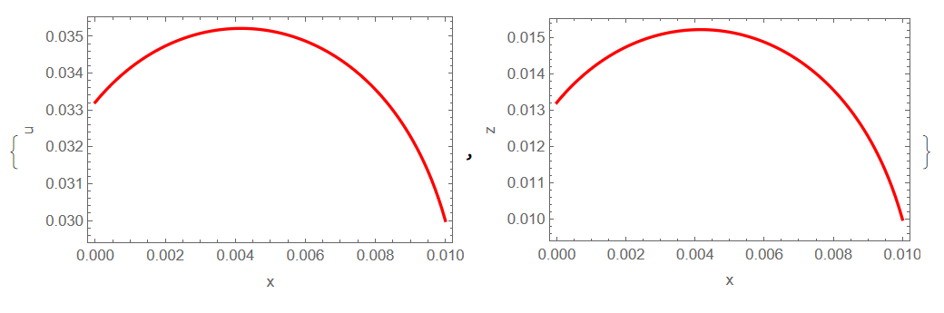
We can also check the quality of this solution in comparison with the wavelet method. Let check $u(a),z(a)$
{u0, z0} = {init[m + 1][[1]], init[m + 1][[2 ]]} Out[]= {0.0332053, 0.0132053} Note that from the Euler wavelets method we have {0.0331914, 0.0131914}. Test for derivatives $u'(a),z'(a)$
rul1 = Table[{u[i] -> init[j][[2 i - 1]], z[i] -> init[j][[2 i]]}, {i, n}] // Flatten; {u1, z1} = {-3 u[1] + 4 u[2] - u[3], -3 z[1] + 4 z[2] - z[3]}/(2 h) /. rul1 Out[]= {1.15472, 1.15469} From wavelets method we have {1.15472, 1.15469}.