z = Transpose@Reverse@Sin@ Outer[Complex, Range[-Pi, Pi, 0.01], Range[-Pi, Pi, 0.01]]; hsbdata = Transpose[{ Rescale[Arg[z], {-Pi, Pi}], 1 - 0.05/Abs[Sin[2 Pi Abs[z]]], 0.02/Abs[Sin[2 Pi Abs[z]]] + Abs[Sin[2 Pi Im@z] Sin[2 Pi Re@z]]^0.25} , {3, 1, 2}]; Image[hsbdata, ColorSpace -> "HSB"] 
EDIT
I wanted to tidy up theThe code and make it easy to produce domain colouring plots of other functionsis below.
The functions defined below are:
complexGrid[max,n] simply generates an $n\times n$ grid of complex numbers ranging from $-max$ to $+max$ in both axes.
complexHSB[Z] takes an array $Z$ of complex numbers and returns an array of $\{h,s,b\}$ values. I've tweaked the colour functions slightly. The initial $\{h,s,b\}$ values are calculated using Heike's formulas, except I don't square $s$. The brightness is then adjusted so that it is high when the saturation is low. The formula is almost the same as $b2=\max (1-s,b)$ but written in a way that makes it Listable.
domainImage[func,max,n] calls the previous two functions to create an image. func is the function to be plotted. The image is generated at twice the desired size and then resized back down to provide a degree of antialiasing.
complexGrid[max,n]simply generates an $n\times n$ grid of complex numbers ranging from $-max$ to $+max$ in both axes.complexHSB[Z]takes an array $Z$ of complex numbers and returns an array of $\{h,s,b\}$ values. I've tweaked the colour functions slightly. The initial $\{h,s,b\}$ values are calculated using Heike's formulas, except I don't square $s$. The brightness is then adjusted so that it is high when the saturation is low. The formula is almost the same as $b2=\max (1-s,b)$ but written in a way that makes itListable.domainImage[func,max,n]calls the previous two functions to create an image.funcis the function to be plotted. The image is generated at twice the desired size and then resized back down to provide a degree of antialiasing.domainPlot[func,max,n]is the end user function which embeds the
image in a graphics frame.
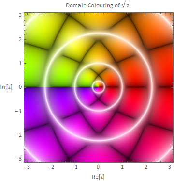
domainPlot[func,max,n] is the end user function. To put tick marks and labels on the final plot I just create an empty ContourPlot and embed the domain colouring image within it. Ideally this should take options which can be passed to ContourPlot but I've never got to grips with option handling so I just put in labels and styles which work for me.
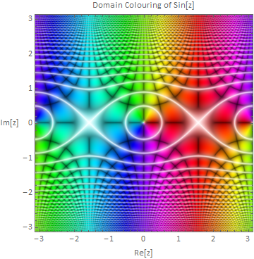
complexGrid = Compile[{{max, _Real}, {n, _Integer}}, Module[Block[{r}, r = Range[-max, max, 2 max/(n - 1)]; Outer[Plus, -I r, r]]]; complexHSB = Compile[{{Z, _Complex, 2}}, Module[Block[{h, s, b, b2}, h = 0.5 +h = Arg[Z]/(2 Pi); s = Abs[Sin[2 Pi Abs[Z]]]; b = Abs[Sin[2Sqrt[Sqrt[Abs[Sin[2 Pi Im[Z]] Sin[2 Pi Re[Z]]]^0.25;Re[Z]]]]]; b2 = 0.5 ((1 - s) + b + Sqrt[(1 - s - b)^2 + 0.01]); Transpose[{h, Sqrt[s], b2}, {3, 1, 2}]]]; domainImage[func_, max_, n_] := ImageResize[ ColorConvert[ImageResize[ColorConvert[ Image[complexHSB@func@complexGrid[max, 2 n], ColorSpace -> "HSB"], "RGB"], n];n, Resampling -> "Gaussian"]; domainPlot[func_: Identity, max_: Pi, n_: 500] := ContourPlot[0, Graphics[{x, -max, max}, {y,Frame -max,> max}True, ContoursPlotRange -> {}max, RotateLabel -> False, FrameLabel -> {"Re[z]", "Im[z]", "Domain Colouring of " <> ToString@StandardForm@func@"z"}, BaseStyle -> {FontFamily -> "Calibri", 1412}, EpilogProlog -> Inset[domainImage[func, max, n], {0, 0}, {Center, Center}, 2` max]]; domainPlot[Sin, Pi] ExamplesOther examples follow:
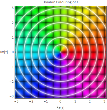
domainPlot[#&];domainPlot[] 

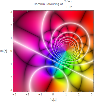
domainPlot[(#+I# + 2 I)/(# - 1) &]