Here's one way to implement Yves's suggestion:
(* arclength function *) trefarc = \[FormalY]\[FormalS] /. First[NDSolve[{\[FormalY]'[t] == Sqrt[#.#] &[D[KnotData[{3, 1}, {\[FormalS]'[t] == Norm[KnotData[{3, 1}, "SpaceCurve"]'[t]], \[FormalS][0] == 0}, "SpaceCurve"][t], t]], \[FormalY][0] == 0}, \[FormalY]\[FormalS], {t, 0, 2 Pi}, Method -> "Extrapolation"]] (* length of trefoil *) end = trefarc[2 Pi]; With[{n = 25}, (* n - number of points to generate *) pts = (KnotData[{3, 1}, "SpaceCurve"][\[FormalT]] /. FindRoot[trefarc[\[FormalT]] == #, {\[FormalT], {\[FormalT], Rescale[#, {0, end}, {0, 2 Pi}], 0, 2 Pi}]) & /@ (end*Range[0, 1, 1/n])] Graphics3D[{Line[pts], AbsolutePointSize[6], Point /@ pts}] 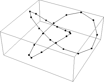
In case the code given above was not sufficiently transparent to readers:
The arclength function
trefarcis produced through the use of Mathematica's numerical differential equation solverNDSolve[](thus yielding anInterpolatingFunction[]suitable for evaluation); recall that the function $s(t)=\int_0^t g(u)\;\mathrm du$ is the solution to the initial value problem $s^\prime(t)=g(t)$, where $g(t)$ is the norm of the derivative of your (plane or space) curve with respect to the parameter.We can use
FindRoot[]for inverting monotonically increasing functions like the arclength function $s(t)$. I used the bracketed form ofFindRoot[],FindRoot[eqn, {var, start, min, max}]to ensure that the algorithms withinFindRoot[]do not go outside the domain of theInterpolatingFunction[]. For the starting point, since the arclength function looks almost like a line, I usedRescale[]to produce the inverse function of the line joining $(0,0)$ and $(2\pi,s(2\pi))$.
Taking a page from Szabolcs's code, the snippet for generating pts can be shortened a fair bit:
With[{n = 25}, pts = Composition[KnotData[{3, 1}, "SpaceCurve"], InverseFunction[trefarc]] /@ (end*Range[0, 1, 1/n])] This hinges on the fact that the InterpolatingFunction[] output by NDSolve[] can be inverted by InverseFunction[].