I have two data sets which go:
datajapan = {{3.22, 0.0149}, {4.7457, 0.06081}, {6.053, 0.1276}, {7.143, 0.211}, {7.9418, 0.3112}, {8.523, 0.411}, {9.322, 0.515}, {9.975, 0.624}, {10.847, 0.736}, {11.50, 0.84}, {12.445, 0.937}, {13.825, 0.94}, {14.48, 0.837}, {14.99, 0.711}, {15.20, 0.587}, {15.57, 0.46}, {16.00, 0.336}, {16.44, 0.211}, {17.167, 0.0984}} JP = ListPlot[datajapan] datajapan2 = {{11.937, -0.031}, {10.629, -0.0853}, {9.467, -0.17}, {8.596, -0.26}, {7.869, -0.356}, {7.2154, -0.469}, {6.489, -0.594}, {5.835, -0.7197}, {5.036, -0.836}, {4.237, -0.94}, {3.365, -1.02}, {2.058, -0.96}, {1.404, -0.8448}, {0.968, -0.719}, {0.75, -0.595}, {0.46, -0.469}, {0.388, -0.302}, {0.315, -0.177}, {-0.121, -0.052}} JP2 = ListPlot[datajapan2] And two equations:
Butler = ParametricNDSolve[{y'[ x] == (kf*(1 - 0.02*ka*Exp[y[x]])*Exp[0.5*(x - y[x])] - kf*0.02*ka*Exp[y[x]]*Exp[0.5*(y[x] - x)])/(10^(-9)*ka* Exp[y[x]]), y[-8] == 0}, y, {x, -8, 19}, {ka, kf}] Butlerback = ParametricNDSolve[{y'[ x] == (kf*(1 - 0.02*ka*Exp[y[x]])*Exp[0.5*(x - y[x])] - kf*0.02*ka*Exp[y[x]]*Exp[0.5*(y[x] - x)])/(-10^(-9)*ka* Exp[y[x]]), y[19] == 3.9 + Log[1/ka]}, y, {x, -8, 19}, {ka, kf}] They have common parameters ka and kf. I need to fit this data with the next equations simultaneously:
(0.130)*ka*Exp[y[ka, kf][x]]*y[ka, kf]'[x]/.Butler -(0.130)*ka*Exp[y[ka, kf][x]]*y[ka, kf]'[x]/.Butlerback I know how to do it by my own hands. I mean, I do following things. Plot these two graphics and datasets together and watch whether they fit each other or not (using some initial parameters):
Show[{Plot[ Evaluate[ Table[-(0.130)*ka*Exp[y[ka, kf][x]]*y[ka, kf]'[x] /. Butlerback, {ka, 0.0001, 0.0011, 0.0002}, {kf, 0.000000015, 0.0000000151, 0.0000000001}]], {x, -8, 19}], Plot[Evaluate[ Table[(0.130)*ka*Exp[y[ka, kf][x]]*y[ka, kf]'[x] /. Butler, {ka, 0.0001, 0.0011, 0.0002}, {kf, 0.000000015, 0.0000000151, 0.0000000001}]], {x, -8, 19}], JP2, JP}, PlotRange -> All] this all looks like this:
 Then I see that I need to increase ka and to decrease kf to it better.
Show[{Plot[ Evaluate[ Table[-(0.130)*ka*Exp[y[ka, kf][x]]*y[ka, kf]'[x] /. Butlerback333, {ka, 0.0083, 0.0085, 0.0002}, {kf, 0.0000000017, 0.00000000171, 0.00000000001}]], {x, -8, 19}], Plot[Evaluate[ Table[(0.130)*ka*Exp[y[ka, kf][x]]*y[ka, kf]'[x] /. Butler333, {ka, 0.0083, 0.0085, 0.0002}, {kf, 0.0000000017, 0.00000000171, 0.00000000001}]], {x, -8, 19}], JP2, JP}, PlotRange -> All] 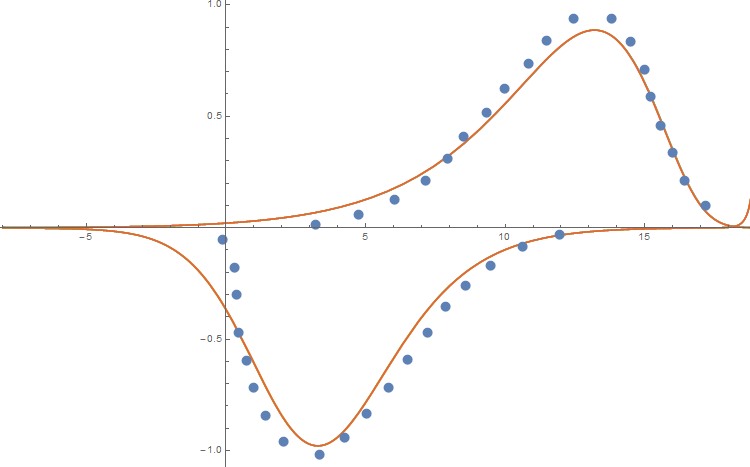
And I change parameters, watch curve again, and again and again till I somehow get a rather good match.
I'd like computer to do it for me, more accurately.
All these calculations are inappropriate because I use wrong initial conditions for Butler (y[-8] is not equal to zero). But this initial condition works somehow so I use it, but I would like computer to take last point of
y[x]/.Butlerbackand use this point as initial condition for Butler
I hope this time i made myself quite clear...)