3
$\begingroup$

I have some data like:

data = Uncompress[FromCharacterCode[ Flatten[ImageData[Import["https://i.sstatic.net/1E5DB.png"], "Byte"]]]] 

If we use FindAnomalies then we can find an outlier:

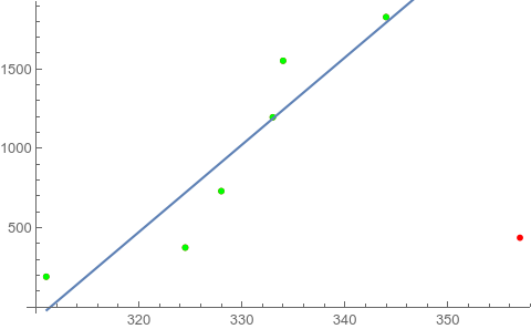
abponts = FindAnomalies[data] 

{{357., 436.5}}

But I don't want to use FindAnomalies to do this, because it is too slow and I don't know how to use other languages to imitate such a neural network function.

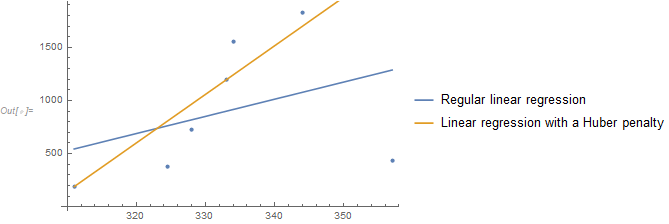
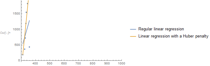
The current idea is to fit a line for all points, then calculate the distance from the point to the fitting line. But it seems like the outlier in data is hard to distinguish as an outlier. The red line is the fitting line in follow:

Show[ListLinePlot[SortBy[data, Last], PlotRange -> {{300, 1000}, {0, 2000}}], Plot[Evaluate[Fit[data, {1, x}, x]], {x, 300, 1000}, PlotStyle -> Red], ListPlot[data, PlotStyle -> Blue]] 

enter image description here

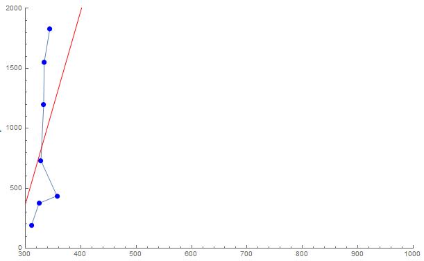
Could anybody can give me some advice?

$\endgroup$
1
  • $\begingroup$ As @JimB says, this is a question for CrossValidated. Maybe look into the RANSAC algorithm? $\endgroup$ Commented Jun 30, 2020 at 5:22

2 Answers 2

9
$\begingroup$

You asked for advice and the best advice is: Consult a statistician. If you can't afford a statistician, ask at CrossValidated.

In any event you should have some reason for tossing out data. That it doesn't look like it fits isn't a good enough reason.

If you have known kinds of errors in the data such as electronic glitches or the coordinates get switched occasionally, then rather than tossing out points you might want to try "robust regression" techniques which reduces the weight of extreme data points (although that's a bit over-generalizing). This goes back to consulting with a statistician.

One of several possibilities with Mathematica is NOT to toss the data but rather give the extreme points less weight in the fitting process.

data = {{311., 191.}, {324.5, 374.5}, {357., 436.5}, {328., 730.5}, {333., 1196.}, {334., 1552.}, {344., 1827.5}}; sol0 = FindFit[data, a + b x, {a, b}, x] (* {a -> -4473.5, b -> 16.1366} *) sol1 = FindFit[data, a + b x, {a, b}, x, NormFunction -> {"HuberPenalty", 0.1}] (* {a -> -14014.8, b -> 45.6779} *) Show[ListPlot[data], Plot[{a + b x /. sol0, a + b x /. sol1}, {x, Min[data[[All, 1]]], Max[data[[All, 1]]]}, PlotLegends -> {"Regular linear regression", "Linear regression with a Huber penalty"}]] 

Data and fits

Using your original scaling:

Show[ListPlot[data, PlotRange -> {{300, 1000}, Automatic}], Plot[{a + b x /. sol0, a + b x /. sol1}, {x, Min[data[[All, 1]]], Max[data[[All, 1]]]}, PlotLegends -> {"Regular linear regression", "Linear regression with a Huber penalty"}]] 

Data and fit with original scaling

$\endgroup$
1
  • $\begingroup$ Thanks for your "robust regression", it is a good thinking.. $\endgroup$ Commented Jun 30, 2020 at 5:01
6
$\begingroup$

I agree that this belongs on CrossValidated because it is about algorithms and not about Mathematica, but nevertheless I'll provide a simple, illustrative example of RANSAC:

computeInliers[{pt1_, pt2_}, pts_, k_ : 1] := Module[{a, b, dist}, {a, b} = Values@FindFit[{pt1, pt2}, a + b x, {a, b}, x]; dist = RegionDistance[InfiniteLine[{pt1, pt2}]] /@ pts; Pick[pts, UnitStep[dist - k StandardDeviation[dist]], 0] ] subsets = Subsets[data, {2}]; inliers = computeInliers[#, data] & /@ subsets; maxSupport = First@MaximalBy[inliers, Length]; line = FindFit[maxSupport, a + b x, {a, b}, x]; Show[ ListPlot[{data, maxSupport}, PlotStyle -> {Red, Green}], Plot[a + b x /. line, {x, 311.`, 357.`}] ] 

Output

$\endgroup$

Start asking to get answers

Find the answer to your question by asking.

Ask question

Explore related questions

See similar questions with these tags.