An InterpolatingFunction has weak singularities at each point of the interpolating grid. They confound the default integration rules, which are a based on the assumption that the integrand is smooth. You can specify the singularities sometimes with Method -> "InterpolationPointsSubdivision", but it does not work here, maybe because of the complexity of p1`. You can also list them explicitly in the iterator that specifies the domain of integration.
sing = Flatten[x["Grid"] /. s1]; (* the interpolation grid *) With[{iter = (* add the relevant singularities to the iterator *) Flatten@{t, 40, Select[sing, 40 < # < 40 + period &], 40 + period}}, paverage = NIntegrate[p1, iter]/period ] (* {-311.513} *) OK, currently this answer has more upvotes than @ChrisK's. While that answer does not explain why it works, it does handle the integral more effectively than my way above. I can explain why.
There are two sources of truncation error in the numerical integration. One comes from the weak singularities that mentioned above. Another, that I mentioned only in a comment, comes from discontinuities in p1 at the points where x'[t] == 0. Further investigation shows these are more significant than the weak singularities I mentioned (and there are 6000+ of them). The setting MaxRecursion -> 100 may seem overkill, but it allows NIntegrate to resolve (quickly, in fact) the error at the discontinuities. The error from the weak singularities does not matter that much because the interpolation grid is so fine that those errors are not that great.
Here's how to see what is going on in Chris's solution:
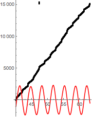
Needs["Integration`NIntegrateUtilities`"] Show[ NIntegrateSamplingPoints@ NIntegrate[p1, {t, 40, 40 + period}, MaxRecursion -> 100], Plot[5000 x'[t] /. s1, {t, 40, 40 + period}, PlotStyle -> Red], PlotRange -> All] 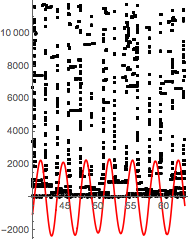
We can see that the sampling is concentrated along the lines where x'[t] == 0. Every now and then the intervals between these roots are subdivided and resampled. This happens when the error from the discontinuities becomes less than the error from the weak singularities (this is the global adaptive strategy). If we do the same analysis on my code, we see that there is very little recursive subdivision with about 50% more sampling points -- and it takes ten times as long. That time can be cut in half with Method -> {"GlobalAdaptive", "SymbolicProcessing" -> 0}.
Show[ With[{iter = Flatten@{t, 40, Select[sing, 40 < # < 40 + period &], 40 + period}}, NIntegrateSamplingPoints@NIntegrate[p1, iter] ], Plot[5000 x'[t] /. s1, {t, 40, 40 + period}, PlotStyle -> Red], PlotRange -> All]