I'm going to brute force it numerically.
First, let's define the function we're interested in:
fun = KnotData[{3, 1}, "SpaceCurve"]
Imagine that this function `fun[t]` describes the position of a moving point in time. The the magnitude of its velocity as a function of the time `t` is
Sqrt[#.#] & [fun'[t]]
I'm going to make an interpolating function out of this to speed up and simplify the numerical calculations:
v = FunctionInterpolation[Sqrt[#.#] & [fun'[t]], {t, 0, 2 Pi}]
The integral (antiderivative) of this function will give us the distance covered as a function of time.
dist = Derivative[-1][v]
This is a monotonically increasing function, so it can be inverted:
invdist = InverseFunction[dist]
Using the inverse we can generate the times at which the point passes through the equally spaced points. Let's divide the curve into 20 equal-length segments:
times = Table[invdist[x], {x, 0, dist[2 Pi], dist[2 Pi]/20}]
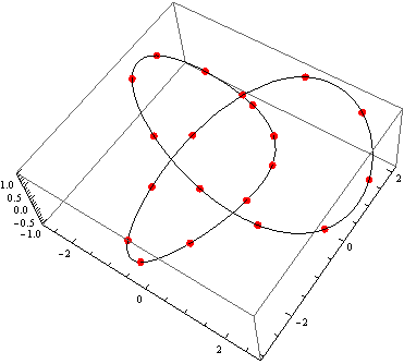
Now we can easily plot the equally spaced points:
Show[
ParametricPlot3D[fun[t], {t, 0, 2 Pi}, PlotStyle -> Black],
ListPointPlot3D[fun /@ times, PlotStyle -> Directive[PointSize[0.02], Red]]
]