Introduction

In this document we give usage examples for the functions of the package, “SystemDynamicsModelGraph.m”, [AAp1]. The package provides functions for making dependency graphs for the stocks in System Dynamics (SD) models. The primary motivation for creating the functions in this package is to have the ability to introspect, proofread, and verify the (typical) ODE models made in SD.

A more detailed explanation is:

• For a given SD system S of Ordinary Differential Equations (ODEs) we make Mathematica graph objects that represent the interaction of variable dependent functions in S.
• Those graph objects give alternative (and hopefully convenient) way of visualizing the model of S.

Load packages

The following commands load the packages [AAp1, AAp2, AAp3]:

Import["https://raw.githubusercontent.com/antononcube/SystemModeling/master/WL/SystemDynamicsModelGraph.m"] Import["https://raw.githubusercontent.com/antononcube/SystemModeling/master/Projects/Coronavirus-propagation-dynamics/WL/EpidemiologyModels.m"] Import["https://raw.githubusercontent.com/antononcube/MathematicaForPrediction/master/Misc/CallGraph.m"]

Usage examples

Equations

Here is a system of ODEs of a slightly modified SEIR model:

lsEqs = {Derivative[1][SP][t] == -((IP[t] SP[t] \[Beta][IP])/TP[t]) - SP[t] \[Mu][TP], Derivative[1][EP][t] == (IP[t] SP[t] \[Beta][IP])/TP[t] - EP[t] (1/aincp + \[Mu][TP]), Derivative[1][IP][t] == EP[t]/aincp - IP[t]/aip - IP[t] \[Mu][IP], Derivative[1][RP][t] == IP[t]/aip - RP[t] \[Mu][TP], TP[t] == Max[0, EP[t] + IP[t] + RP[t] + SP[t]]}; ResourceFunction["GridTableForm"][List /@ lsEqs, TableHeadings -> {"Equations"}]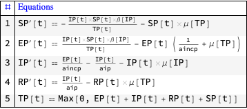

Model graph

Here is a graph of the dependencies between the populations:

ModelDependencyGraph[lsEqs, {EP, IP, RP, SP, TP}, t]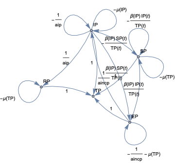

When the second argument given to ModelDependencyGraph is Automatic the stocks in the equations are heuristically found with the function ModelHeuristicStocks:

ModelHeuristicStocks[lsEqs, t]  (*{EP, IP, RP, SP, TP}*)

Also, the function ModelDependencyGraph takes all options of Graph:

ModelDependencyGraph[lsEqs, Automatic, t,   GraphLayout -> "GravityEmbedding", VertexLabels -> "Name", VertexLabelStyle -> Directive[Red, Bold, 16], EdgeLabelStyle -> Directive[Blue, 16], ImageSize -> Large]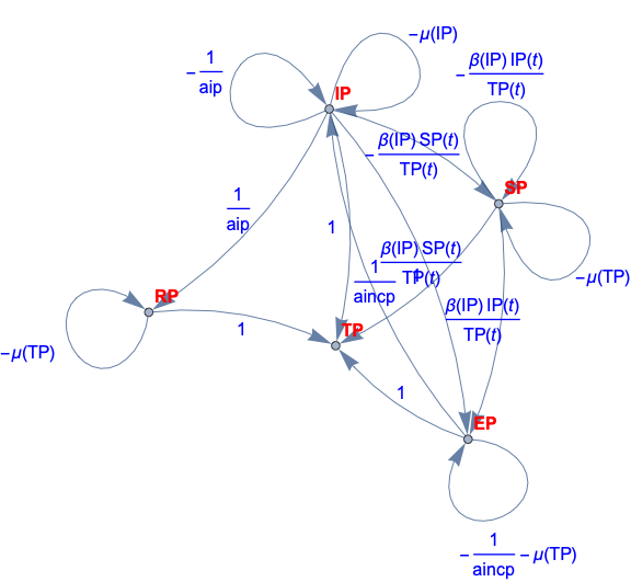

Dependencies only

The dependencies in the model can be found with the function ModelDependencyGraphEdges:

lsEdges = ModelDependencyGraphEdges[lsEqs, Automatic, t]

lsEdges[[4]] // FullForm

Focus stocks

Here is a graph for a set of “focus” stocks-sources to a set of “focus” stocks-destinations:

gr = ModelDependencyGraph[lsEqs, {IP, SP}, {EP}, t]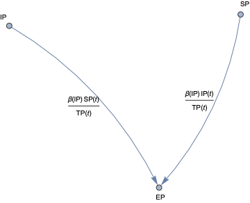

Compare with the graph in which the argument positions of sources and destinations of the previous command are swapped:

ModelDependencyGraph[lsEqs, {EP}, {IP, SP}, t]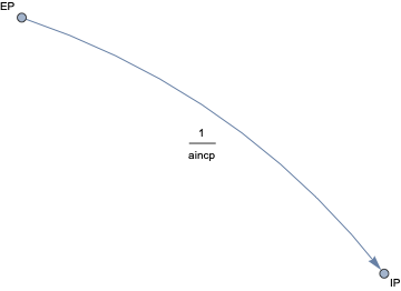

Additional interfacing

The functions of this package work with the models from the package “EpidemiologyModels.m”, [AAp2].

Here is a model from [AAp2]:

model = SEIRModel[t, "TotalPopulationRepresentation" -> "AlgebraicEquation"]; ModelGridTableForm[model]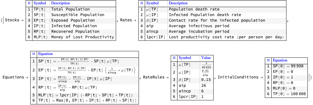

Here we make the corresponding graph:

ModelDependencyGraph[model, t]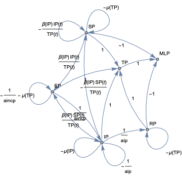

Generating equations from graph specifications

A related, dual, or inverse task to the generation of graphs from systems of ODEs is the generation of system of ODEs from graphs.

Here is a model specifications through graph edges (using DirectedEdge):

Here is the corresponding graph:

grModel = Graph[lsEdges, VertexLabels -> "Name", EdgeLabels -> "EdgeTag", ImageSize -> Large]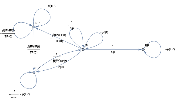

Here we generate the system of ODEs using the function ModelGraphEquations:

lsEqsGen = ModelGraphEquations[grModel, t]; ResourceFunction["GridTableForm"][List /@ lsEqsGen, TableHeadings -> {"Equations"}]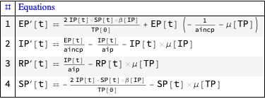

Remark: ModelGraphEquations works with both graph and list of edges as a first argument.

Here we replace the symbolically represented rates with concrete values:

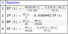
Here we solve the system of ODEs:

sol = First@NDSolve[{lsEqsGen2, SP[0] == 99998, EP[0] == 0, IP[0] == 1, RP[0] == 0,MLP[0] == 0, TP[0] == 100000}, Union[First /@ lsEdges], {t, 0, 365}]

Here we plot the results:

ListLinePlot[sol[[All, 2]], PlotLegends -> sol[[All, 1]]]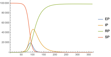

Call graph

The functionalities provided by the presented package “SystemDynamicsModelGraph.m”, [AAp1], resemble in spirit those of the package “CallGraph.m”, [AAp3].

Here is call graph for the functions in the package [AAp1] made with the function CallGraph from the package [AAp3]:

CallGraph`CallGraph[Context[ModelDependencyGraph], "PrivateContexts" -> False, "UsageTooltips" -> True]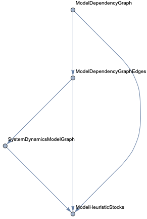

References

Packages

[AAp1] Anton Antonov, “System Dynamics Model Graph Mathematica package”, (2020), SystemsModeling at GitHub/antononcube.

[AAp2] Anton Antonov, “Epidemiology models Mathematica package”, (2020), SystemsModeling at GitHub/antononcube.

[AAp3] Anton Antonov, “Call graph generation for context functions Mathematica package”, (2018), MathematicaForPrediction at GitHub/antononcube.

Articles

[AA1] Anton Antonov, “Call graph generation for context functions”, (2019), MathematicaForPrediction at WordPress.