Introduction

In this document we describe the design and implementation of a (software programming) monad for Quantile Regression workflows specification and execution. The design and implementation are done with Mathematica / Wolfram Language (WL).

What is Quantile Regression? : Assume we have a set of two dimensional points each point being a pair of an independent variable value and a dependent variable value. We want to find a curve that is a function of the independent variable that splits the points in such a way that, say, 30% of the points are above that curve. This is done with Quantile Regression, see [Wk2, CN1, AA2, AA3]. Quantile Regression is a method to estimate the variable relations for all parts of the distribution. (Not just, say, the mean of the relationships found with Least Squares Regression.)

The goal of the monad design is to make the specification of Quantile Regression workflows (relatively) easy, straightforward, by following a certain main scenario and specifying variations over that scenario. Since Quantile Regression is often compared with Least Squares Regression and some type of filtering (like, Moving Average) those functionalities should be included in the monad design scenarios.

The monad is named QRMon and it is based on the State monad package "StateMonadCodeGenerator.m", [AAp1, AA1] and the Quantile Regression package "QuantileRegression.m", [AAp4, AA2].

The data for this document is read from WL’s repository or created ad-hoc.

The monadic programming design is used as a Software Design Pattern. The QRMon monad can be also seen as a Domain Specific Language (DSL) for the specification and programming of machine learning classification workflows.

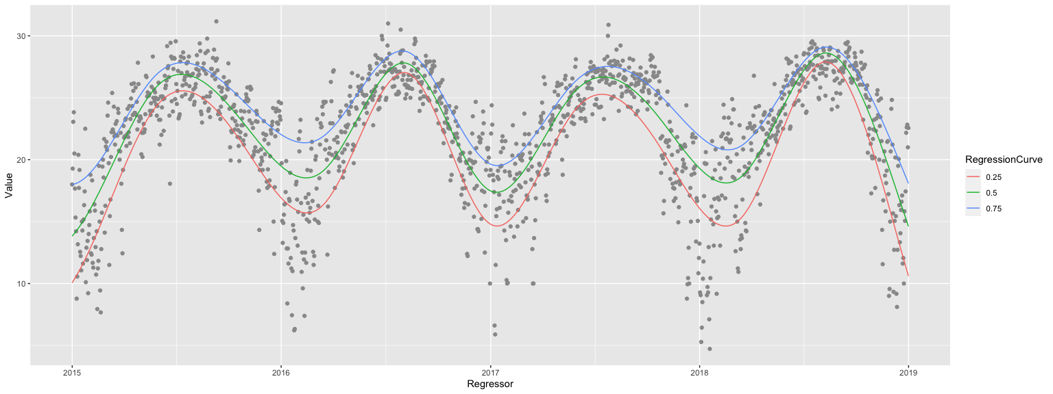
Here is an example of using the QRMon monad over heteroscedastic data::

The table above is produced with the package "MonadicTracing.m", [AAp2, AA1], and some of the explanations below also utilize that package.

As it was mentioned above the monad QRMon can be seen as a DSL. Because of this the monad pipelines made with QRMon are sometimes called "specifications".

Remark: With "regression quantile" we mean "a curve or function that is computed with Quantile Regression".

Contents description

The document has the following structure.

• The sections "Package load" and "Data load" obtain the needed code and data.
  • (Needed and put upfront from the "Reproducible research" point of view.)
• The sections "Design consideration" and "Monad design" provide motivation and design decisions rationale.

• The sections "QRMon overview" and "Monad elements" provide technical description of the QRMon monad needed to utilize it.

  • (Using a fair amount of examples.)
• The section "Unit tests" describes the tests used in the development of the QRMon monad.
  • (The random pipelines unit tests are especially interesting.)
• The section "Future plans" outlines future directions of development.
  • (The most interesting and important one is the "conversational agent" direction.)
• The section "Implementation notes" just says that QRMon’s development process and this document follow the ones of the classifications workflows monad ClCon, [AA6].

Remark: One can read only the sections "Introduction", "Design consideration", "Monad design", and "QRMon overview". That set of sections provide a fairly good, programming language agnostic exposition of the substance and novel ideas of this document.

The table above is produced with the package "MonadicTracing.m", [AAp2, AA1], and some of the explanations below also utilize that package.

As it was mentioned above the monad QRMon can be seen as a DSL. Because of this the monad pipelines made with QRMon are sometimes called "specifications".

Remark: With "regression quantile" we mean "a curve or function that is computed with Quantile Regression".

Package load

The following commands load the packages [AAp1–AAp6]:

Import["https://raw.githubusercontent.com/antononcube/\ MathematicaForPrediction/master/MonadicProgramming/\ MonadicQuantileRegression.m"] Import["https://raw.githubusercontent.com/antononcube/\ MathematicaForPrediction/master/MonadicProgramming/MonadicTracing.m"]

Data load

In this section we load data that is used in the rest of the document. The time series data is obtained through WL’s repository.

The data summarization and plots are done through QRMon, which in turn uses the function RecordsSummary from the package "MathematicaForPredictionUtilities.m", [AAp6].

Distribution data

The following data is generated to have [heteroscedasticity(https://en.wikipedia.org/wiki/Heteroscedasticity).

distData = Table[{x, Exp[-x^2] + RandomVariate[ NormalDistribution[0, .15 Sqrt[Abs[1.5 - x]/1.5]]]}, {x, -3, 3, .01}]; Length[distData] (* 601 *) QRMonUnit[distData]⟹QRMonEchoDataSummary⟹QRMonPlot;

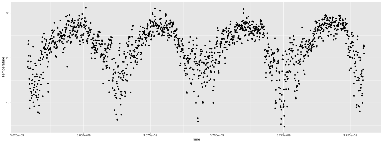
Temperature time series

tsData = WeatherData[{"Orlando", "USA"}, "Temperature", {{2015, 1, 1}, {2018, 1, 1}, "Day"}] QRMonUnit[tsData]⟹QRMonEchoDataSummary⟹QRMonDateListPlot;

Financial time series

The following data is typical for financial time series. (Note the differences with the temperature time series.)

finData = TimeSeries[FinancialData["NYSE:GE", {{2014, 1, 1}, {2018, 1, 1}, "Day"}]]; QRMonUnit[finData]⟹QRMonEchoDataSummary⟹QRMonDateListPlot;

Design considerations

The steps of the main regression workflow addressed in this document follow.

1. Retrieving data from a data repository.

2. Optionally, transform the data.

   1. Delete rows with missing fields.

   2. Rescale data along one or both of the axes.

   3. Apply moving average (or median, or map.)

3. Verify assumptions of the data.

4. Run a regression algorithm with a certain basis of functions using:

   1. Quantile Regression, or

   2. Least Squares Regression.

5. Visualize the data and regression functions.

6. If the regression functions fit is not satisfactory go to step 4.

7. Utilize the found regression functions to compute:

   1. outliers,

   2. local extrema,

   3. approximation or fitting errors,

   4. conditional density distributions,

   5. time series simulations.

The following flow-chart corresponds to the list of steps above.

In order to address:

• the introduction of new elements in regression workflows,

• workflows elements variability, and

• workflows iterative changes and refining,

it is beneficial to have a DSL for regression workflows. We choose to make such a DSL through a functional programming monad, [Wk1, AA1].

Here is a quote from [Wk1] that fairly well describes why we choose to make a classification workflow monad and hints on the desired properties of such a monad.

[…] The monad represents computations with a sequential structure: a monad defines what it means to chain operations together. This enables the programmer to build pipelines that process data in a series of steps (i.e. a series of actions applied to the data), in which each action is decorated with the additional processing rules provided by the monad. […] Monads allow a programming style where programs are written by putting together highly composable parts, combining in flexible ways the possible actions that can work on a particular type of data. […]

Remark: Note that quote from [Wk1] refers to chained monadic operations as "pipelines". We use the terms "monad pipeline" and "pipeline" below.

Monad design

The monad we consider is designed to speed-up the programming of quantile regression workflows outlined in the previous section. The monad is named QRMon for "Quantile Regression Monad".

We want to be able to construct monad pipelines of the general form:

QRMon is based on the State monad, [Wk1, AA1], so the monad pipeline form (1) has the following more specific form:

This means that some monad operations will not just change the pipeline value but they will also change the pipeline context.

In the monad pipelines of QRMon we store different objects in the contexts for at least one of the following two reasons.

1. The object will be needed later on in the pipeline, or

2. The object is (relatively) hard to compute.

Such objects are transformed data, regression functions, and outliers.

Let us list the desired properties of the monad.

• Rapid specification of non-trivial quantile regression workflows.

• The monad works with time series, numerical matrices, and numerical vectors.

• The pipeline values can be of different types. Most monad functions modify the pipeline value; some modify the context; some just echo results.

• The monad can do quantile regression with B-Splines bases, quantile regression fit and least squares fit with specified bases of functions.

• The monad allows of cursory examination and summarization of the data.

• It is easy to obtain the pipeline value, context, and different context objects for manipulation outside of the monad.

• It is easy to plot different combinations of data, regression functions, outliers, approximation errors, etc.

The QRMon components and their interactions are fairly simple.

The main QRMon operations implicitly put in the context or utilize from the context the following objects:

• (time series) data,

• regression functions,

• outliers and outlier regression functions.

Note the that the monadic set of types of QRMon pipeline values is fairly heterogenous and certain awareness of "the current pipeline value" is assumed when composing QRMon pipelines.

Obviously, we can put in the context any object through the generic operations of the State monad of the package "StateMonadGenerator.m", [AAp1].

QRMon overview

When using a monad we lift certain data into the "monad space", using monad’s operations we navigate computations in that space, and at some point we take results from it.

With the approach taken in this document the "lifting" into the QRMon monad is done with the function QRMonUnit. Results from the monad can be obtained with the functions QRMonTakeValue, QRMonContext, or with the other QRMon functions with the prefix "QRMonTake" (see below.)

Here is a corresponding diagram of a generic computation with the QRMon monad:

Remark: It is a good idea to compare the diagram with formulas (1) and (2).

Let us examine a concrete QRMon pipeline that corresponds to the diagram above. In the following table each pipeline operation is combined together with a short explanation and the context keys after its execution.

Here is the output of the pipeline:

The QRMon functions are separated into four groups:

• operations,

• setters and droppers,

• takers,

• State Monad generic functions.

An overview of the those functions is given in the tables in next two sub-sections. The next section, "Monad elements", gives details and examples for the usage of the QRMon operations.

Monad functions interaction with the pipeline value and context

The following table gives an overview the interaction of the QRMon monad functions with the pipeline value and context.

The following table shows the functions that are function synonyms or short-cuts.

State monad functions

Here are the QRMon State Monad functions (generated using the prefix "QRMon", [AAp1, AA1]):

Monad elements

In this section we show that QRMon has all of the properties listed in the previous section.

The monad head

The monad head is QRMon. Anything wrapped in QRMon can serve as monad’s pipeline value. It is better though to use the constructor QRMonUnit. (Which adheres to the definition in [Wk1].)

QRMon[{{1, 223}, {2, 323}}, <||>]⟹QRMonEchoDataSummary;

Lifting data to the monad

The function lifting the data into the monad QRMon is QRMonUnit.

The lifting to the monad marks the beginning of the monadic pipeline. It can be done with data or without data. Examples follow.

QRMonUnit[distData]⟹QRMonEchoDataSummary;

QRMonUnit[]⟹QRMonSetData[distData]⟹QRMonEchoDataSummary;

(See the sub-section "Setters, droppers, and takers" for more details of setting and taking values in QRMon contexts.)

Currently the monad can deal with data in the following forms:

• time series,

• numerical vectors,

• numerical matrices of rank two.

When the data lifted to the monad is a numerical vector vec it is assumed that vec has to become the second column of a "time series" matrix; the first column is derived with Range[Length[vec]] .

Generally, WL makes it easy to extract columns datasets order to obtain numerical matrices, so datasets are not currently supported in QRMon.

Quantile regression with B-splines

This computes quantile regression with B-spline basis over 12 regularly spaced knots. (Using Linear Programming algorithms; see [AA2] for details.)

QRMonUnit[distData]⟹ QRMonQuantileRegression[12]⟹ QRMonPlot;

The monad function QRMonQuantileRegression has the same options as QuantileRegression. (The default value for option Method is different, since using "CLP" is generally faster.)

Options[QRMonQuantileRegression] (* {InterpolationOrder -> 3, Method -> {LinearProgramming, Method -> "CLP"}} *)

Let us compute regression using a list of particular knots, specified quantiles, and the method "InteriorPoint" (instead of the Linear Programming library CLP):

p = QRMonUnit[distData]⟹ QRMonQuantileRegression[{-3, -2, 1, 0, 1, 1.5, 2.5, 3}, Range[0.1, 0.9, 0.2], Method -> {LinearProgramming, Method -> "InteriorPoint"}]⟹ QRMonPlot;

Remark: As it was mentioned above the function QRMonRegression is a synonym of QRMonQuantileRegression.

The fit functions can be extracted from the monad with QRMonTakeRegressionFunctions, which gives an association of quantiles and pure functions.

ListPlot[# /@ distData[[All, 1]]] & /@ (p⟹QRMonTakeRegressionFunctions)

Quantile regression fit and Least squares fit

Instead of using a B-spline basis of functions we can compute a fit with our own basis of functions.

Here is a basis functions:

bFuncs = Table[PDF[NormalDistribution[m, 1], x], {m, Min[distData[[All, 1]]], Max[distData[[All, 1]]], 1}]; Plot[bFuncs, {x, Min[distData[[All, 1]]], Max[distData[[All, 1]]]}, PlotRange -> All, PlotTheme -> "Scientific"]

Here we do a Quantile Regression fit, a Least Squares fit, and plot the results:

p = QRMonUnit[distData]⟹ QRMonQuantileRegressionFit[bFuncs]⟹ QRMonLeastSquaresFit[bFuncs]⟹ QRMonPlot; 

Remark: The functions "QRMon*Fit" should generally have a second argument for the symbol of the basis functions independent variable. Often that symbol can be omitted and implied. (Which can be seen in the pipeline above.)

Remark: As it was mentioned above the function QRMonRegressionFit is a synonym of QRMonQuantileRegressionFit and QRMonFit is a synonym of QRMonLeastSquaresFit.

As it was pointed out in the previous sub-section, the fit functions can be extracted from the monad with QRMonTakeRegressionFunctions. Here the keys of the returned/taken association consist of quantiles and "mean" since we applied both Quantile Regression and Least Squares Regression.

ListPlot[# /@ distData[[All, 1]]] & /@ (p⟹QRMonTakeRegressionFunctions)

Default basis to fit (using Chebyshev polynomials)

One of the main advantages of using the function QuanileRegression of the package [AAp4] is that the functions used to do the regression with are specified with a few numeric parameters. (Most often only the number of knots is sufficient.) This is achieved by using a basis of B-spline functions of a certain interpolation order.

We want similar behaviour for Quantile Regression fitting we need to select a certain well known basis with certain desirable properties. Such basis is given by Chebyshev polynomials of first kind [Wk3]. Chebyshev polynomials bases can be easily generated in Mathematica with the functions ChebyshevT or ChebyshevU.

Here is an application of fitting with a basis of 12 Chebyshev polynomials of first kind:

QRMonUnit[distData]⟹ QRMonQuantileRegressionFit[12]⟹ QRMonLeastSquaresFit[12]⟹ QRMonPlot;

The code above is equivalent to the following code:

bfuncs = Table[ChebyshevT[i, Rescale[x, MinMax[distData[[All, 1]]], {-0.95, 0.95}]], {i, 0, 12}]; p = QRMonUnit[distData]⟹ QRMonQuantileRegressionFit[bfuncs]⟹ QRMonLeastSquaresFit[bfuncs]⟹ QRMonPlot;

The shrinking of the ChebyshevT domain seen in the definitions of bfuncs is done in order to prevent approximation error effects at the ends of the data domain. The following code uses the ChebyshevT domain { − 1, 1} instead of the domain { − 0.95, 0.95} used above.

QRMonUnit[distData]⟹ QRMonQuantileRegressionFit[{4, {-1, 1}}]⟹ QRMonPlot;

Regression functions evaluation

The computed quantile and least squares regression functions can be evaluated with the monad function QRMonEvaluate.

Evaluation for a given value of the independent variable:

p⟹QRMonEvaluate[0.12]⟹QRMonTakeValue (* <|0.25 -> 0.930402, 0.5 -> 1.01411, 0.75 -> 1.08075, "mean" -> 0.996963|> *)

Evaluation for a vector of values:

p⟹QRMonEvaluate[Range[-1, 1, 0.5]]⟹QRMonTakeValue (* <|0.25 -> {0.258241, 0.677461, 0.943299, 0.703812, 0.293741}, 0.5 -> {0.350025, 0.768617, 1.02311, 0.807879, 0.374545}, 0.75 -> {0.499338, 0.912183, 1.10325, 0.856729, 0.431227}, "mean" -> {0.355353, 0.776006, 1.01118, 0.783304, 0.363172}|> *)

Evaluation for complicated lists of numbers:

p⟹QRMonEvaluate[{0, 1, {1.5, 1.4}}]⟹QRMonTakeValue (* <|0.25 -> {0.943299, 0.293741, {0.0762883, 0.10759}}, 0.5 -> {1.02311, 0.374545, {0.103386, 0.139142}}, 0.75 -> {1.10325, 0.431227, {0.133755, 0.177161}}, "mean" -> {1.01118, 0.363172, {0.107989, 0.142021}}|> *) 

The obtained values can be used to compute estimates of the distributions of the dependent variable. See the sub-sections "Estimating conditional distributions" and "Dependent variable simulation".

Errors and error plots

Here with "errors" we mean the differences between data’s dependent variable values and the corresponding values calculated with the fitted regression curves.

In the pipeline below we compute couple of regression quantiles, plot them together with the data, we plot the errors, compute the errors, and summarize them.

QRMonUnit[finData]⟹ QRMonQuantileRegression[10, {0.5, 0.1}]⟹ QRMonDateListPlot[Joined -> False]⟹ QRMonErrorPlots["DateListPlot" -> True, Joined -> False]⟹ QRMonErrors⟹ QRMonEchoFunctionValue["Errors summary:", RecordsSummary[#[[All, 2]]] & /@ # &];

Each of the functions QRMonErrors and QRMonErrorPlots computes the errors. (That computation is considered cheap.)

Finding outliers

Finding outliers can be done with the function QRMonOultiers. The outliers found by QRMonOutliers are simply points that below or above certain regression quantile curves, for example, the ones corresponding to 0.02 and 0.98.

Here is an example:

p = QRMonUnit[distData]⟹ QRMonQuantileRegression[6, {0.02, 0.98}]⟹ QRMonOutliers⟹ QRMonEchoValue⟹ QRMonOutliersPlot;

The function QRMonOutliers puts in the context values for the keys "outliers" and "outlierRegressionFunctions". The former is for the found outliers, the latter is for the functions corresponding to the used regression quantiles.

Keys[p⟹QRMonTakeContext] (* {"data", "regressionFunctions", "outliers", "outlierRegressionFunctions"} *)

Here are the corresponding quantiles of the plot above:

Keys[p⟹QRMonTakeOutlierRegressionFunctions] (* {0.02, 0.98} *)

The control of the outliers computation is done though the arguments and options of QRMonQuantileRegression (or the rest of the regression calculation functions.)

If only one regression quantile is found in the context and the corresponding quantile is less than 0.5 then QRMonOutliers finds only bottom outliers. If only one regression quantile is found in the context and the corresponding quantile is greater than 0.5 then QRMonOutliers finds only top outliers.

Here is an example for finding only the top outliers:

QRMonUnit[finData]⟹ QRMonQuantileRegression[5, 0.8]⟹ QRMonOutliers⟹ QRMonEchoFunctionContext["outlier quantiles:", Keys[#outlierRegressionFunctions] &]⟹ QRMonOutliersPlot["DateListPlot" -> True]; 

Plotting outliers

The function QRMonOutliersPlot makes an outliers plot. If the outliers are not in the context then QRMonOutliersPlot calls QRMonOutliers first.

Here are the options of QRMonOutliersPlot:

Options[QRMonOutliersPlot] (* {"Echo" -> True, "DateListPlot" -> False, ListPlot -> {Joined -> False}, Plot -> {}} *)

The default behavior is to echo the plot. That can be suppressed with the option "Echo".

QRMonOutliersPlot utilizes combines with Show two plots:

• one with ListPlot (or DateListPlot) for the data and the outliers,

• the other with Plot for the regression quantiles used to find the outliers.

That is why separate lists of options can be given to manipulate those two plots. The option DateListPlot can be used make plots with date or time axes.

QRMonUnit[tsData]⟹ QRMonQuantileRegression[12, {0.01, 0.99}]⟹ QRMonOutliersPlot[ "Echo" -> False, "DateListPlot" -> True, ListPlot -> {PlotStyle -> {Green, {PointSize[0.02], Red}, {PointSize[0.02], Blue}}, Joined -> False, PlotTheme -> "Grid"}, Plot -> {PlotStyle -> Orange}]⟹ QRMonTakeValue 

Estimating conditional distributions

Consider the following problem:

How to estimate the conditional density of the dependent variable given a value of the conditioning independent variable?

(In other words, find the distribution of the y-values for a given, fixed x-value.)

The solution of this problem using Quantile Regression is discussed in detail in [PG1] and [AA4].

Finding a solution for this problem can be seen as a primary motivation to develop Quantile Regression algorithms.

The following pipeline (i) computes and plots a set of five regression quantiles and (ii) then using the found regression quantiles computes and plots the conditional distributions for two focus points (−2 and 1.)

QRMonUnit[distData]⟹ QRMonQuantileRegression[6, Range[0.1, 0.9, 0.2]]⟹ QRMonPlot[GridLines -> {{-2, 1}, None}]⟹ QRMonConditionalCDF[{-2, 1}]⟹ QRMonConditionalCDFPlot;

Moving average, moving median, and moving map

Fairly often it is a good idea for a given time series to apply filter functions like Moving Average or Moving Median. We might want to:

• visualize the obtained transformed data,

• do regression over the transformed data,

• compare with regression curves over the original data.

For these reasons QRMon has the functions QRMonMovingAverage, QRMonMovingMedian, and QRMonMovingMap that correspond to the built-in functions MovingAverage, MovingMedian, and MovingMap.

Here is an example:

QRMonUnit[tsData]⟹ QRMonDateListPlot[ImageSize -> Small]⟹ QRMonMovingAverage[20]⟹ QRMonEchoFunctionValue["Moving avg: ", DateListPlot[#, ImageSize -> Small] &]⟹ QRMonMovingMap[Mean, Quantity[20, "Days"]]⟹ QRMonEchoFunctionValue["Moving map: ", DateListPlot[#, ImageSize -> Small] &];

Dependent variable simulation

Consider the problem of making a time series that is a simulation of a process given with a known time series.

More formally,

• we are given a time-axis grid (regular or irregular),

• we consider each grid node to correspond to a random variable,

• we want to generate time series based on the empirical CDF’s of the random variables that correspond to the grid nodes.

The formulation of the problem hints to an (almost) straightforward implementation using Quantile Regression.

p = QRMonUnit[tsData]⟹QRMonQuantileRegression[30, Join[{0.01}, Range[0.1, 0.9, 0.1], {0.99}]]; tsNew = p⟹ QRMonSimulate[1000]⟹ QRMonTakeValue; opts = {ImageSize -> Medium, PlotTheme -> "Detailed"}; GraphicsGrid[{{DateListPlot[tsData, PlotLabel -> "Actual", opts], DateListPlot[tsNew, PlotLabel -> "Simulated", opts]}}]

Finding local extrema in noisy data

Using regression fitting — and Quantile Regression in particular — we can easily construct semi-symbolic algorithms for finding local extrema in noisy time series data; see [AA5]. The QRMon function with such an algorithm is QRMonLocalExtrema.

In brief, the algorithm steps are as follows. (For more details see [AA5].)

1. Fit a polynomial through the data.

2. Find the local extrema of the fitted polynomial. (We will call them fit estimated extrema.)

3. Around each of the fit estimated extrema find the most extreme point in the data by a nearest neighbors search (by using Nearest).

The function QRMonLocalExtrema uses the regression quantiles previously found in the monad pipeline (and stored in the context.) The bottom regression quantile is used for finding local minima, the top regression quantile is used for finding the local maxima.

An example of finding local extrema follows.

QRMonUnit[TimeSeriesWindow[tsData, {{2015, 1, 1}, {2018, 12, 31}}]]⟹ QRMonQuantileRegression[10, {0.05, 0.95}]⟹ QRMonDateListPlot[Joined -> False, PlotTheme -> "Scientific"]⟹ QRMonLocalExtrema["NumberOfProximityPoints" -> 100]⟹ QRMonEchoValue⟹ QRMonAddToContext⟹ QRMonEchoFunctionContext[ DateListPlot[{#localMinima, #localMaxima, #data}, PlotStyle -> {PointSize[0.015], PointSize[0.015], Gray}, Joined -> False, PlotLegends -> {"localMinima", "localMaxima", "data"}, PlotTheme -> "Scientific"] &];

Note that in the pipeline above in order to plot the data and local extrema together some additional steps are needed. The result of QRMonLocalExtrema becomes the pipeline value; that pipeline value is displayed with QRMonEchoValue, and stored in the context with QRMonAddToContext. If the pipeline value is an association — which is the case here — the monad function QRMonAddToContext joins that association with the context association. In this case this means that we will have key-value elements in the context for "localMinima" and "localMaxima". The date list plot at the end of the pipeline uses values of those context keys (together with the value for "data".)

Setters, droppers, and takers

The values from the monad context can be set, obtained, or dropped with the corresponding "setter", "dropper", and "taker" functions as summarized in a previous section.

For example:

p = QRMonUnit[distData]⟹QRMonQuantileRegressionFit[2]; p⟹QRMonTakeRegressionFunctions (* <|0.25 -> (0.0191185 + 0.00669159 #1 + 3.05509*10^-14 #1^2 &), 0.5 -> (0.191408 + 9.4728*10^-14 #1 + 3.02272*10^-14 #1^2 &), 0.75 -> (0.563422 + 3.8079*10^-11 #1 + 7.63637*10^-14 #1^2 &)|> *) 

If other values are put in the context they can be obtained through the (generic) function QRMonTakeContext, [AAp1]:

p = QRMonUnit[RandomReal[1, {2, 2}]]⟹QRMonAddToContext["data"]; (p⟹QRMonTakeContext)["data"] (* {{0.608789, 0.741599}, {0.877074, 0.861554}} *)

Another generic function from [AAp1] is QRMonTakeValue (used many times above.)

Here is an example of the "data dropper" QRMonDropData:

p⟹QRMonDropData⟹QRMonTakeContext (* <||> *)

(The "droppers" simply use the state monad function QRMonDropFromContext, [AAp1]. For example, QRMonDropData is equivalent to QRMonDropFromContext["data"].)

Unit tests

The development of QRMon was done with two types of unit tests: (i) directly specified tests, [AAp7], and (ii) tests based on randomly generated pipelines, [AA8].

The unit test package should be further extended in order to provide better coverage of the functionalities and illustrate — and postulate — pipeline behavior.

Directly specified tests

Here we run the unit tests file "MonadicQuantileRegression-Unit-Tests.wlt", [AAp7]:

AbsoluteTiming[ testObject = TestReport["~/MathematicaForPrediction/UnitTests/MonadicQuantileRegression-Unit-Tests.wlt"] ]

The natural language derived test ID’s should give a fairly good idea of the functionalities covered in [AAp3].

Values[Map[#["TestID"] &, testObject["TestResults"]]] (* {"LoadPackage", "GenerateData", "QuantileRegression-1", \ "QuantileRegression-2", "QuantileRegression-3", \ "QuantileRegression-and-Fit-1", "Fit-and-QuantileRegression-1", \ "QuantileRegressionFit-and-Fit-1", "Fit-and-QuantileRegressionFit-1", \ "Outliers-1", "Outliers-2", "GridSequence-1", "BandsSequence-1", \ "ConditionalCDF-1", "Evaluate-1", "Evaluate-2", "Evaluate-3", \ "Simulate-1", "Simulate-2", "Simulate-3"} *)

Random pipelines tests

Since the monad QRMon is a DSL it is natural to test it with a large number of randomly generated "sentences" of that DSL. For the QRMon DSL the sentences are QRMon pipelines. The package "MonadicQuantileRegressionRandomPipelinesUnitTests.m", [AAp8], has functions for generation of QRMon random pipelines and running them as verification tests. A short example follows.

Generate pipelines:

SeedRandom[234] pipelines = MakeQRMonRandomPipelines[100]; Length[pipelines] (* 100 *)

Here is a sample of the generated pipelines:

(* Block[{DoubleLongRightArrow, pipelines = RandomSample[pipelines, 6]}, Clear[DoubleLongRightArrow]; pipelines = pipelines /. {_TemporalData -> "tsData", _?MatrixQ -> "distData"}; GridTableForm[Map[List@ToString[DoubleLongRightArrow @@ #, FormatType -> StandardForm] &, pipelines], TableHeadings -> {"pipeline"}] ] AutoCollapse[] *)

Here we run the pipelines as unit tests:

AbsoluteTiming[ res = TestRunQRMonPipelines[pipelines, "Echo" -> False]; ]

From the test report results we see that a dozen tests failed with messages, all of the rest passed.

rpTRObj = TestReport[res]

(The message failures, of course, have to be examined — some bugs were found in that way. Currently the actual test messages are expected.)

Future plans

Workflow operations

A list of possible, additional workflow operations and improvements follows.

• Certain improvements can be done over the specification of the different plot options.

• It will be useful to develop a function for automatic finding of over-fitting parameters.

• The time series simulation should be done by aggregation of similar time intervals.

  • For example, for time series with span several years, for each month name is made Quantile Regression simulation and the results are spliced to obtain a one year simulation.
• If the time series is represented as a sequence of categorical values, then the time series simulation can use Bayesian probabilities derived from sub-sequences.
  • QRMon already has functions that facilitate that, QRMonGridSequence and QRMonBandsSequence.

Conversational agent

Using the packages [AAp10, AAp11] we can generate QRMon pipelines with natural commands. The plan is to develop and document those functionalities further.

Here is an example of a pipeline constructed with natural language commands:

QRMonUnit[distData]⟹ ToQRMonPipelineFunction["show data summary"]⟹ ToQRMonPipelineFunction["calculate quantile regression for quantiles 0.2, 0.8 and with 40 knots"]⟹ ToQRMonPipelineFunction["plot"];

Implementation notes

The implementation methodology of the QRMon monad packages [AAp3, AAp8] followed the methodology created for the ClCon monad package [AAp9, AA6]. Similarly, this document closely follows the structure and exposition of the ClCon monad document "A monad for classification workflows", [AA6].

A lot of the functionalities and signatures of QRMon were designed and programed through considerations of natural language commands specifications given to a specialized conversational agent. (As discussed in the previous section.)

References

Packages

[AAp1] Anton Antonov, State monad code generator Mathematica package, (2017), MathematicaForPrediction at GitHub. URL: https://github.com/antononcube/MathematicaForPrediction/blob/master/MonadicProgramming/StateMonadCodeGenerator.m .

[AAp2] Anton Antonov, Monadic tracing Mathematica package, (2017), MathematicaForPrediction at GitHub. URL: https://github.com/antononcube/MathematicaForPrediction/blob/master/MonadicProgramming/MonadicTracing.m .

[AAp3] Anton Antonov, Monadic Quantile Regression Mathematica package, (2018), MathematicaForPrediction at GitHub. URL: https://github.com/antononcube/MathematicaForPrediction/blob/master/MonadicProgramming/MonadicQuantileRegression.m.

[AAp4] Anton Antonov, Quantile regression Mathematica package, (2014), MathematicaForPrediction at GitHub. URL: https://github.com/antononcube/MathematicaForPrediction/blob/master/QuantileRegression.m .

[AAp5] Anton Antonov, Monadic contextual classification Mathematica package, (2017), MathematicaForPrediction at GitHub. URL: https://github.com/antononcube/MathematicaForPrediction/blob/master/MonadicProgramming/MonadicContextualClassification.m .

[AAp6] Anton Antonov, MathematicaForPrediction utilities, (2014), MathematicaForPrediction at GitHub. URL: https://github.com/antononcube/MathematicaForPrediction/blob/master/MathematicaForPredictionUtilities.m .

[AAp7] Anton Antonov, Monadic Quantile Regression unit tests, (2018), MathematicaVsR at GitHub. URL: https://github.com/antononcube/MathematicaForPrediction/blob/master/UnitTests/MonadicQuantileRegression-Unit-Tests.wlt .

[AAp8] Anton Antonov, Monadic Quantile Regression random pipelines Mathematica unit tests, (2018), MathematicaForPrediction at GitHub. URL: https://github.com/antononcube/MathematicaForPrediction/blob/master/UnitTests/MonadicQuantileRegressionRandomPipelinesUnitTests.m .

[AAp9] Anton Antonov, Monadic contextual classification Mathematica package, (2017), MathematicaForPrediction at GitHub. URL: https://github.com/antononcube/MathematicaForPrediction/blob/master/MonadicProgramming/MonadicContextualClassification.m .

ConversationalAgents Packages

[AAp10] Anton Antonov, Time series workflows grammar in EBNF, (2018), ConversationalAgents at GitHub, https://github.com/antononcube/ConversationalAgents.

[AAp11] Anton Antonov, QRMon translator Mathematica package,(2018), ConversationalAgents at GitHub, https://github.com/antononcube/ConversationalAgents.

MathematicaForPrediction articles

[AA1] Anton Antonov, "Monad code generation and extension", (2017), MathematicaForPrediction at GitHub, https://github.com/antononcube/MathematicaForPrediction.

[AA2] Anton Antonov, "Quantile regression through linear programming", (2013), MathematicaForPrediction at WordPress. URL: https://mathematicaforprediction.wordpress.com/2013/12/16/quantile-regression-through-linear-programming/ .

[AA3] Anton Antonov, "Quantile regression with B-splines", (2014), MathematicaForPrediction at WordPress. URL: https://mathematicaforprediction.wordpress.com/2014/01/01/quantile-regression-with-b-splines/ .

[AA4] Anton Antonov, "Estimation of conditional density distributions", (2014), MathematicaForPrediction at WordPress. URL: https://mathematicaforprediction.wordpress.com/2014/01/13/estimation-of-conditional-density-distributions/ .

[AA5] Anton Antonov, "Finding local extrema in noisy data using Quantile Regression", (2015), MathematicaForPrediction at WordPress. URL: https://mathematicaforprediction.wordpress.com/2015/09/27/finding-local-extrema-in-noisy-data-using-quantile-regression/ .

[AA6] Anton Antonov, "A monad for classification workflows", (2018), MathematicaForPrediction at WordPress. URL: https://mathematicaforprediction.wordpress.com/2018/05/15/a-monad-for-classification-workflows/ .

Other

[Wk1] Wikipedia entry, Monad, URL: https://en.wikipedia.org/wiki/Monad_(functional_programming) .

[Wk2] Wikipedia entry, Quantile Regression, URL: https://en.wikipedia.org/wiki/Quantile_regression .

[Wk3] Wikipedia entry, Chebyshev polynomials, URL: https://en.wikipedia.org/wiki/Chebyshev_polynomials .

[CN1] Brian S. Code and Barry R. Noon, "A gentle introduction to quantile regression for ecologists", (2003). Frontiers in Ecology and the Environment. 1 (8): 412[Dash]420. doi:10.2307/3868138. URL: http://www.econ.uiuc.edu/~roger/research/rq/QReco.pdf .

[PS1] Patrick Scheibe, Mathematica (Wolfram Language) support for IntelliJ IDEA, (2013-2018), Mathematica-IntelliJ-Plugin at GitHub. URL: https://github.com/halirutan/Mathematica-IntelliJ-Plugin .

[RK1] Roger Koenker, Quantile Regression, ‪Cambridge University Press, 2005‬.