I am trying to numerically solve equation (6) of Lakhina 2021 in Python. The equation is
$$\frac{1}{2}\left(\frac{d \phi}{d\xi}\right)^2 + S(\phi, M) = 0\, .$$
The Sagdeev potential expression is given by (7).
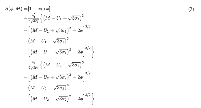
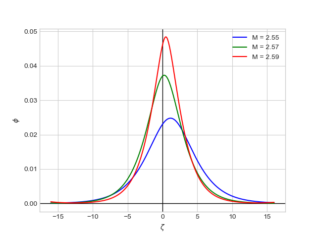
What I want is to reproduce the potential profiles in Fig. 3 of Lakhina 2021.
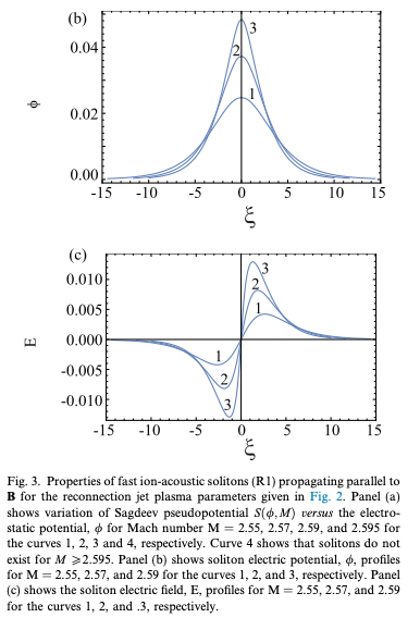
The boundary conditions given in the paper are:
$\phi(0)_{M = 2.55} = 0.023$
$\phi(0)_{M = 2.57} = 0.037$
$\phi(0)_{M = 2.55} = 0.046$
In the code below, I first define a function for the first-order differential equation. Then, set boundary conditions for each mach number, $M$, and finally, I use odeint from the scipy.integrate module in Python to solve the boundary value problem. The plot of the solutions is shown in the last figure.
Here is my attempt, the Python code:
## Importing standard modules from scipy.integrate import odeint import numpy as np import matplotlib.pyplot as plt ## Reconnection jet plasma parameters n1 = 0.74 n2 = 0.26 sig1 = 0.11 sig2 = 0.07 U1 = -1.72 U2 = 1.82 # Function for Sagdeev potential equation def S(phi, M): s = (1 - np.exp(phi)) + n1/(6*np.sqrt(3*sig1))*((M - U1 + np.sqrt(3*sig1))**3 - ((M - U1 + np.sqrt(3*sig1))**2 - 2*phi)**1.5 - (M - U1 - np.sqrt(3*sig1))**3 + ((M - U1 - np.sqrt(3*sig1))**2 - 2*phi)**1.5) + n2/(6*np.sqrt(3*sig2))*( (M - U2 + np.sqrt(3*sig2))**3 - ((M - U2 + np.sqrt(3*sig2))**2 - 2*phi)**1.5 - (M - U2 - np.sqrt(3*sig2))**3 + ((M - U2 - np.sqrt(3*sig2))**2 - 2*phi)**1.5) return s ## Solving the ode def model(phi, zeta, M): S = (1 - np.exp(phi)) + n1/(6*np.sqrt(3*sig1))*((M - U1 + np.sqrt(3*sig1))**3 - ((M - U1 + np.sqrt(3*sig1))**2 - 2*phi)**1.5 - (M - U1 - np.sqrt(3*sig1))**3 + ((M - U1 - np.sqrt(3*sig1))**2 - 2*phi)**1.5) + n2/(6*np.sqrt(3*sig2))*( (M - U2 + np.sqrt(3*sig2))**3 - ((M - U2 + np.sqrt(3*sig2))**2 - 2*phi)**1.5 - (M - U2 - np.sqrt(3*sig2))**3 + ((M - U2 - np.sqrt(3*sig2))**2 - 2*phi)**1.5) dphi_dzeta = -np.sqrt(-2*S) return dphi_dzeta # Boundary conditions phi0_M255 = 0.023 #For M = 2.55 phi0_M257 = 0.037 #For M = 2.57 phi0_M259 = 0.046 #For M = 2.59 phi_array = np.linspace(-0.01, 0.06, 1000) zeta_array = np.linspace(-16, 16, 1000) Phi = odeint(model, phi0, zeta_array, args = (2.57,)) ## Plotting plt.figure(2) plt.axhline(0, color = 'k', lw = 1) plt.axvline(0, color = 'k', lw = 1) plt.plot(zeta_array, Phi, label = "M = 2.55") plt.xlabel("$\zeta$") plt.ylabel("S($\phi$, M)") plt.legend() Output:
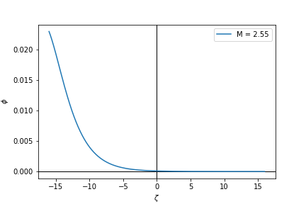
May you please assist? I am really not sure where I am going wrong.
References
- Lakhina, G. S., Singh, S. V., & Rubia, R. (2021). A mechanism for electrostatic solitary waves observed in the reconnection jet region of the Earth’s magnetotail. Advances in Space Research.
odeintis targeted to initial value problems. $\endgroup$