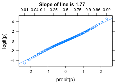
@Benoit Sanchez and @gung's graphs emphasize how little there is to distinguish the link functions, except with very large numbers of observations and/or in the extreme tails. The conversion ${\rm logit}(p) = 1.77\ {\rm probit}(p)$ never has an error of more than $0.1$ over the range $0.1 \le p \le 0.9$. Over $0.01 \le p \le 0.99$, the conversion is still a good approximation. Using such a conversion factor, one can get a good approximation to the odds ratio from a model that has a probit link.
The graph uses the following R code:
trellis.par.set(clip=list(panel='off')) p <- (1:99)/100 logit <- make.link('logit')$linkfun probit <- make.link('probit')$linkfun gph <- lattice::xyplot(logit(p)~probit(p), type=c('p','r'), scales=list(x=list(alternating=1, tck=c(0.6,0)))) b <- coef(lm(logit(p) ~ 0 + probit(p))) ## Slope of line gph1 <- update(gph, main = list(paste("Slope of line is", round(b,2)), cex=1)) probs <- c(.01,.0504,.1, .25,.5,.75,.9,.9596,.99) gph+latticeExtragph1+latticeExtra::layer(panel.axis(side='top', at=probit(probs), labels=paste(probs),outside=T, rot=0))