You seem to be asking about a nonparametric estimator for the mean.
First, let's make it clear: for Bayesian statistics, you always need to make distributional assumptions. You can proceed as suggested by Sextus Empiricus (+1), but this does assume Gaussian distribution. If you really didn't want to make any assumptions, in practice, you would probably just estimate the arithmetic mean.
But let's try coming up with a nonparametric solution. One thing that comes to my mind is Bayesian bootstrap also described by Rasmus Bååth who provided code example. With Bayesian bootstrap, you would assume the Dirichlet-uniform distribution for the probabilities, resample with replacement the datapoints and evaluate the statistic, so arithmetic mean on those samples. But in such a case, to approximate the frequentist estimator, you would use the same estimator on the samples to find their distribution. Not very helpful, isn't it?
Let's start again. The definition of expected value is
$$ E[X] = \int x \, f(x)\, dx $$
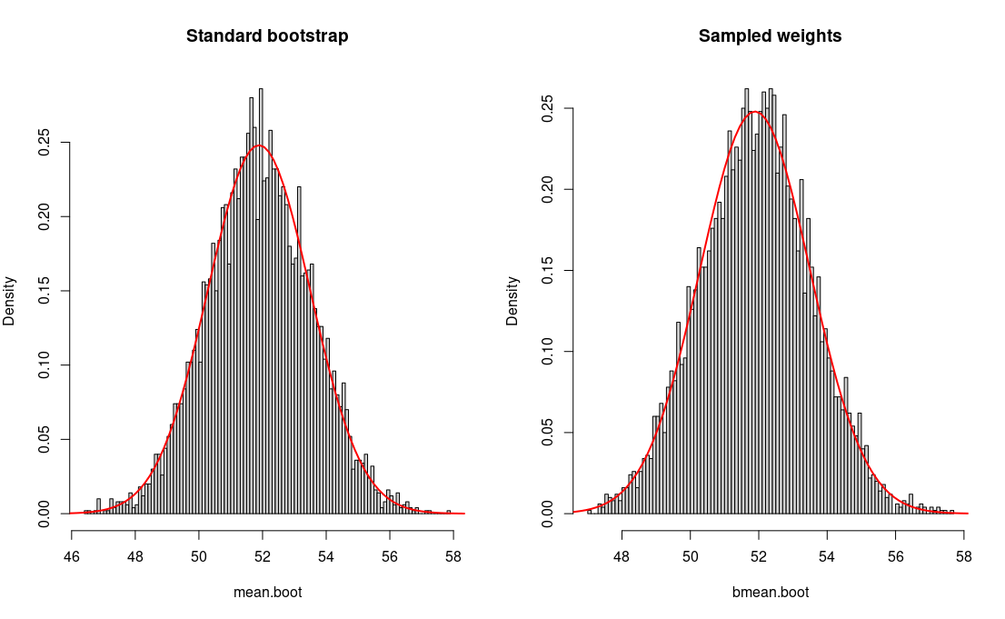
The problem is that you don't know the probability densities $f(x)$. In the frequentist setting, it is estimated using the arithmetic average. It is in fact a weighted average, where weights are empirical probabilities. Same as with Bayesian bootstrap, you could use a prior for them by drawing them from Dirichlet-uniform distribution, calculating the weighted average, and repeating this many times to find the distribution of the estimates. If you think about it, It's the most trivial case of the Bayesian bootstrap for a weighted statistic. As you can read from the links provided above, this makes a number of unreasonable assumptions like approximating continuous distribution with a discrete one. Not that it is very useful, but if you insist on a Bayesian nonparametric estimator, that's a possibility. As you can see from the example below, it gives the same results as the frequentist estimator and standard bootstrap.
set.seed(42) N <- 500 X <- rnorm(N, 53, 37) mean(x) ## [1] 51.88829 R <- 5000 mean.boot <- replicate(R, mean(sample(X, replace=TRUE))) summary(mean.boot) ## Min. 1st Qu. Median Mean 3rd Qu. Max. ## 46.41 50.81 51.90 51.91 53.03 57.88 bmean.boot <- replicate(R, weighted.mean(X, w=rexp(N, 1))) summary(bmean.boot) ## Min. 1st Qu. Median Mean 3rd Qu. Max. ## 47.09 50.82 51.93 51.91 52.99 57.65 par(mfrow=c(1, 2)) hist(mean.boot, 100, freq=FALSE, main="Standard bootstrap") curve(dnorm(x, mean(X), sd(X)/sqrt(N)), 45, 60, add=T, col="red", lw=2) hist(bmean.boot, 100, freq=FALSE, main="Sampled weights") curve(dnorm(x, mean(X), sd(X)/sqrt(N)), 45, 60, add=T, col="red", lw=2)