There are simple relationships for the bounds of $\lambda$ where you get all coefficients zero and where you get none of the coefficients zero.
LASSO: Deriving the smallest lambda at which all coefficient are zero $$\lambda_{\text{all zero}} = \sqrt{k} \vert \vert X^T y\vert \vert_\infty$$
What is the smallest $\lambda$ that gives a 0 component in lasso? $$\lambda_{\text{non zero}} = \frac{d}{n} \vert \vert X \vec{\beta}_{last,normalized} \vert \vert_2^2 $$ with $$\vec{\beta}_{last,normalized} = \frac{\vec{\beta}_{last}}{\sum \vec{\beta}_{last} \cdot sign(\hat{\beta})} $$ and $$\vec{\beta}_{last} = - (X^TX)^{-1} \text{sign} (\hat{\beta}) $$
A demonstration of the above formula's with some code
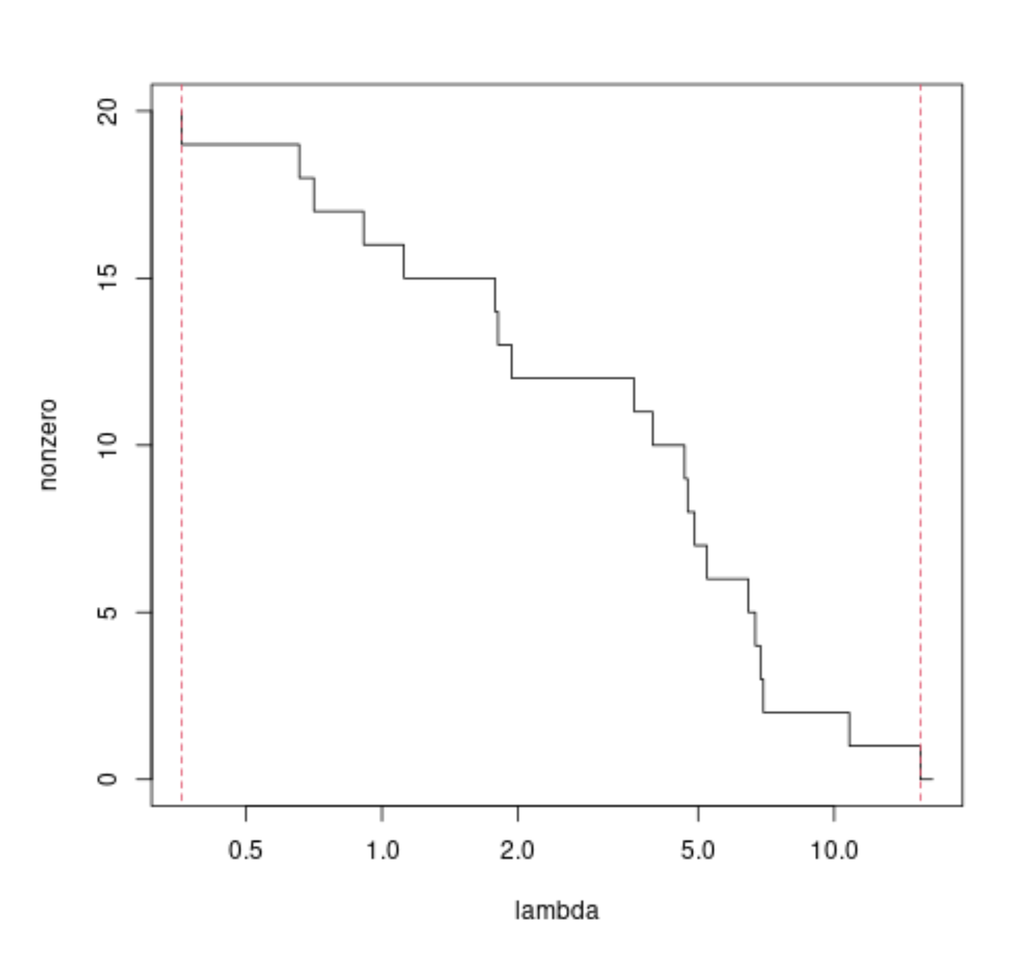
library(lars) ### generate some data set.seed(1) n = 50 m = 20 X = matrix(rnorm(m*n),n) y = rnorm(n) ### perform lasso mod = lars(X,y, intercept = 0, normalize = 0) nonzero = rowSums(mod$beta^2 > 0) lambda = mod$lambda lambda = c(lambda[1]+1,lambda) # add one additional point ### plot the number of nonzero estimated coefficients ### as function of lambda plot(lambda,nonzero, log ="x", type = "s") ### upper bound above which all coefficients are zero l_max = max(abs(t(X) %*% y)) lines(l_max*c(1,1), c(-1,m+1), lty = 2, col = 2) ### lower bound below which all coefficients are non-zero mod = lm(y~0+X) beta = mod$coefficients bl = - solve(t(X)%*%X) %*% sign(beta) bln = bl/sum(bl*sign(beta)) br = beta/bln d = min(br[br>0]) l_min = sum((X %*% bln)^2)*d lines(l_min*c(1,1), c(-1,m+1), lty = 2, col = 2) A simple algorithm to compute the path of solutions to LASSO is least angle regression.
A difficulty to compute directly the value of the penalty $\lambda$ where a particular coefficient becomes non-zero is that it depends on which other coëfficiënts are already non-zero.
This is because of correlations between the coefficients, which makes that the increase of one coefficient can reduce the effect of another. For example one may get even a situation where a coefficient reduces in magnitude as we decrease the penalty (Why under joint least squares direction is it possible for some coefficients to decrease in LARS regression?). Sometimes a coefficient can change from positive to negative (cross zero) as we change the penalty parameter (https://stats.stackexchange.com/a/594633/) and the number of non-zero components as function of the penalty parameter can be a non-monotonic function.
It is easy to compute the points in the paths when either:
We only look at the beginning or the end, as is done in this answer.
When there are no correlations between the regressors, as is done in the answer by EdM.