A known difference between fitting an exponential curve with a nonlinear fitting or with a linearized fitting is the difference in the relevance of the error/residuals of different points.
You can notice this in the plot below.
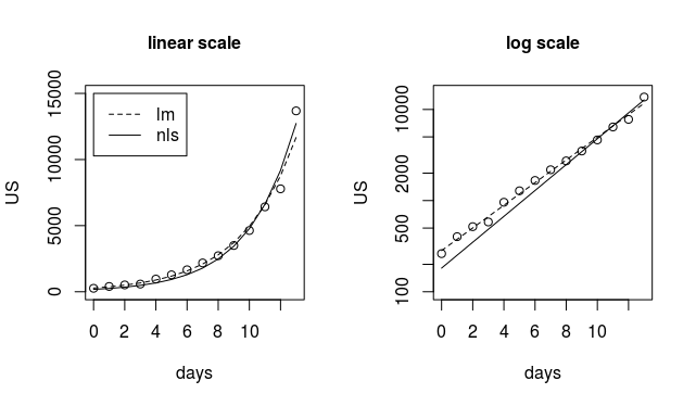
In that plot you can see that
- the linearized fit (the broken line) is fitting more precisely the points with small values (see the plot on the right where the broken line is closer to the values in the beginning).
the non linear fit is closer to the points with high values.
modnls <- nls(US ~ a*exp(b*days), start=list(a=100, b=0.3)) modlm <- lm(log(US) ~ days ) plot(days,US, ylim = c(1,15000)) lines(days,predict(modnls)) lines(days,exp(predict(modlm)), lty=2) title("linear scale", cex.main=1) legend(0,15000,c("lm","nls"),lty=c(2,1)) plot(days,US, log = "y", ylim = c(100,15000)) lines(days,predict(modnls)) lines(days,exp(predict(modlm)), lty=2) title("log scale", cex.main=1)
Getting the random noise modeled correctly is not always right in practice
In practice the problem is not so often what sort of model to use for the random noise (whether it should be some sort of glm or not).
The problem is much more that the exponential model (the deterministic part) is not correct, and the choice of fitting a linearized model or not is a choice in the strength between the first points versus fitting the last points. The linearized model fits very well the values at a small size and the non-linear model fits better the values with high values.
You can see the incorrectness of the exponential model when we plot the ratio of increase.
When we plot the ratio of the increase, for the world variable, as function of time, then you can see that it is a non-constant variable (and for this period it appears to be increasing). You can make the same plot for the US but it is very noisy, that is because the numbers are still small and differentiating a noisy curve makes the noise:signal ratio larger.
(also note that the error terms will be incremental and if you really wish to do it right then you should use some arima type of model for the error, or use some other way to make the error terms correlated)

I still don't get why lm with log gives me completely different coefficients. How do I convert between the two?
The glm and nls model the errors both as $$y−y_{model}∼N(0,\sigma^2)$$ The linearized model models the errors as $$log(y)−log(y_{model})∼N(0,\sigma^2)$$ but when you take the logarithm of values then you change the relative size. The difference between 1000.1 and 1000 and 1.1 and 1 is both 0.1. But on a log scale it is not the same difference anymore.
This is actually how the glm does the fitting. It uses a linear model, but with transformed weigths for the errors (and it iterates this a few times). See the following two which return the same result:
last_14 <- list(days <- 0:13, World <- c(101784,105821,109795, 113561,118592,125865,128343,145193,156094,167446,181527,197142,214910,242708), US <- c(262,402,518,583,959,1281,1663,2179,2727,3499,4632,6421,7783,13677)) days <- last_14[[1]] US<- last_14[[3]] World <- last_14[[2]] Y <- log(US) X <- cbind(rep(1,14),days) coef <- lm.fit(x=X, y=Y)$coefficients yp <- exp(X %*% coef) for (i in 1:100) { # itterating with different # weights w <- as.numeric(yp^2) # y-values Y <- log(US) + (US-yp)/yp # solve weighted linear equation coef <- solve(crossprod(X,w*X), crossprod(X,w*Y)) # If am using lm.fit then for some reason you get something different then direct matrix solution # lm.wfit(x=X, y=Y, w=w)$coefficients yp <- exp(X %*% coef) } coef # > coef # [,1] # 5.2028935 # days 0.3267964 glm(US ~days, family = gaussian(link = "log"), control = list(epsilon = 10^-20, maxit = 100)) # > glm(US ~days, # + family = gaussian(link = "log"), # + control = list(epsilon = 10^-20, maxit = 100)) # # Call: glm(formula = US ~ days, family = gaussian(link = "log"), control = list(epsilon = 10^-20, # maxit = 100)) # # Coefficients: # (Intercept) days # 5.2029 0.3268 # # Degrees of Freedom: 13 Total (i.e. Null); 12 Residual # Null Deviance: 185900000 # Residual Deviance: 3533000 AIC: 219.9
nlsyou can try using the formula $$a \cdot \text{exp} (b \cdot \text{days})$$ instead of $$ \text{exp} (b \cdot \text{days})$$ For instance, this code will work:nls(World ~ a*exp(b*days), last_14, start=list(a=100000, b=0.3))$\endgroup$