Fuzzy clustering allows each data point to belong to multiple clusters with different membership values. Instead of assigning a point to just one group, it captures how strongly a point relates to each cluster.
- Uses membership scores between 0 and 1
- Handles overlapping or unclear cluster boundaries
- More flexible than hard clustering methods
- Useful when data points don’t fit neatly into a single group
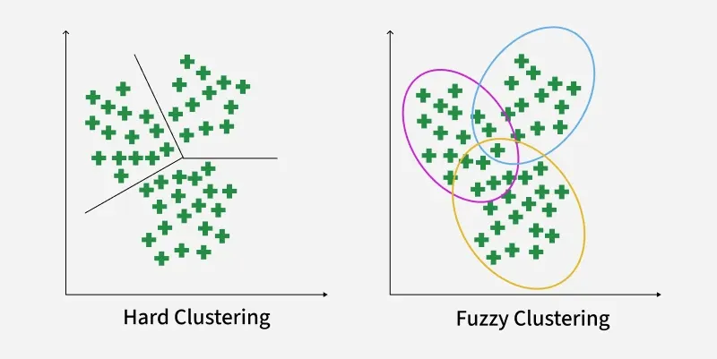 Hard Clustering vs Fuzzy Clustering
Working of Fuzzy Clustering
Fuzzy clustering assigns each data point a degree of membership for every cluster and updates these values through an iterative process. Here’s how it works:
Step 1: Initialize Membership Values Randomly: Each data point is given random membership scores for all clusters. A point can partially belong to multiple clusters.
For example, for 2 clusters and 4 data points, an initial membership matrix (\gamma) might look like:
Cluster | (1,3) | (2,5) | (4,8) | (7,9) |
|---|
1 | 0.8 | 0.7 | 0.2 | 0.1 |
|---|
2 | 0.2 | 0.3 | 0.8 | 0.9 |
|---|
Step 2: Compute Cluster Centroids: Centroids are calculated as weighted averages, where weights are membership values raised to the fuzziness parameter m:
V_{ij} = \frac{\sum_{k=1}^{n} \gamma_{ik}^m \cdot x_{kj}} {\sum_{k=1}^{n} \gamma_{ik}^m}
Where:
- \gamma_{ik} = membership of point k in cluster i.
- m = fuzziness parameter (usually 2).
- x_{kj} = value of feature j for point k.
Step 3: Calculate Distance Between Data Points and Centroids: Compute the Euclidean distance between each point and every centroid to determine proximity, which will be used to update memberships. Example for point (1,3):
D_{11} = \sqrt{(1 - 1.568)^2 + (3 - 4.051)^2} = 1.2
D_{12} = \sqrt{(1 - 5.35)^2 + (3 - 8.215)^2} = 6.79
Similarly the distance of all other points is computed from both the centroids.
Step 4: Update Membership Values: Membership values are updated inversely proportional to these distances. Points closer to a centroid get higher membership.
Updated membership \gamma_{ik} for point k in cluster i is:
\gamma = \sum \limits_1^n {(d_{ki}^2 /d_{kj}^2)}^{1/m-1} ]^{-1}
Step 5: Repeat Until Convergence: Steps 2–4 are repeated until the membership values stabilize meaning there are no significant changes from one iteration to the next. This indicates that the clustering has reached an optimal state.
Implementation of Fuzzy Clustering
The fuzzy scikit learn library has a pre-defined function for fuzzy c-means which can be used in Python. For using fuzzy c-means we need to install the skfuzzy library.
pip install scikit-fuzzy
Step 1: Importing Libraries
We will use numpy for numerical operations, skfuzzy for the Fuzzy C-Means clustering algorithm and matplotlib for plotting the results.
Python import numpy as np import skfuzzy as fuzz import matplotlib.pyplot as plt
Step 2: Generating Sample Data
We will creates 100 two-dimensional points clustered using Gaussian noise.
- Set random seed (np.random.seed(0)): Ensures results are reproducible every time you run the code.
- Define center = 0.5 and spread = 0.1: The cluster points will be centered around 0.5 with some variation.
- Generate data (np.random.randn(2, 100)): Creates 100 random points in 2D space using Gaussian (normal) distribution.
- Clip values (np.clip(data, 0, 1)): Ensures all points lie within the [0,1] range (keeps data bounded).
Python np.random.seed(0) center = 0.5 spread = 0.1 data = center + spread * np.random.randn(2, 100) data = np.clip(data, 0, 1)
Step 3: Setting Fuzzy C-Means Parameters
Parameters control clustering behavior: number of clusters, fuzziness degree, stop tolerance and max iterations for convergence.
- n_clusters = 3: We want to divide data into 3 clusters.
- m = 1.7: The fuzziness parameter; higher values make cluster memberships softer (points can belong to multiple clusters).
- error = 1e-5: The stopping tolerance; algorithm stops if changes are smaller than this threshold.
- maxiter = 2000: The maximum number of iterations allowed to reach convergence.
Python n_clusters = 3 m = 1.7 error = 1e-5 maxiter = 2000
Step 4: Performing Fuzzy C-Means Clustering and Assign Each Point to a Hard Cluster
Converts fuzzy memberships to hard cluster assignments by taking the cluster with highest membership for each point.
- cntr: Final cluster centers
- u: Membership matrix indicating degree of belonging for each point to each cluster
- fpc: Fuzzy partition coefficient (quality metric)
This runs the clustering algorithm on the data.
Python cntr, u, _, _, _, _, fpc = fuzz.cluster.cmeans( data, c=n_clusters, m=m, error=error, maxiter=maxiter, init=None ) hard_clusters = np.argmax(u, axis=0)
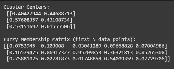
Step 5: Printing Cluster Centers and Membership Matrix
Outputs coordinates of cluster centers and the membership values for the first 5 data points to provide insight into clustering results.
Python print("Cluster Centers:\n", cntr) print("\nFuzzy Membership Matrix (first 5 data points):") print(u[:, :5]) Output:
 Cluster
Step 6: Visualizing Fuzzy Memberships and Hard Clusters
Plots membership levels as soft-colored points and overlays crisp cluster assignments with distinct markers to visualize both fuzzy and hard clustering. Cluster centers are highlighted with red X marks.
Python fig, ax = plt.subplots(figsize=(8, 6)) for i in range(n_clusters): ax.scatter(data[0], data[1], c=u[i], cmap='coolwarm', alpha=0.5, label=f'Fuzzy Cluster {i+1}') markers = ['o', 's', '^'] colors = ['blue', 'green', 'orange'] for i in range(n_clusters): cluster_points = data[:, hard_clusters == i] ax.scatter(cluster_points[0], cluster_points[1], c=colors[i], marker=markers[i], edgecolor='k', s=80, label=f'Hard Cluster {i+1}') ax.scatter(cntr[:, 0], cntr[:, 1], c='red', marker='X', s=200, label='Cluster Centers') ax.set_title('Fuzzy C-Means') ax.set_xlabel('Feature 1') ax.set_ylabel('Feature 2') ax.legend(loc='upper left') plt.grid(True) plt.show() Output:
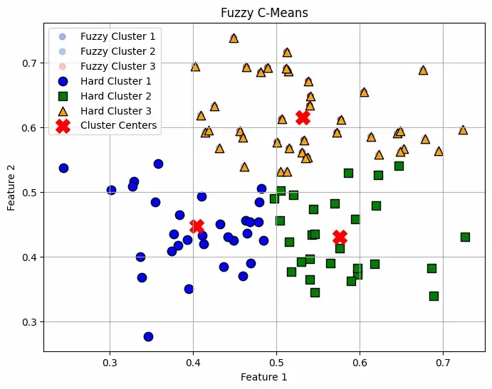 Fuzzy C-Mean Plotting
The plot shows soft clustering meaning a point can belong to multiple clusters with different probabilities rather than being assigned to just one cluster. This makes it useful when boundaries between clusters are not well-defined and all the Red "X" markers indicate the cluster centers computed by the algorithm.
You Can Download the complete code from here.
Applications
- Image Segmentation: Handles noise and overlapping regions efficiently.
- Pattern Recognition: Identifies ambiguous patterns in speech, handwriting, etc.
- Customer Segmentation: Groups customers with partial membership for flexible marketing.
- Medical Diagnosis: Analyzes patient or genetic data with uncertain boundaries.
- Bioinformatics: Captures multifunctional gene roles by assigning genes to multiple clusters.
Advantages
- Flexibility: Allows overlapping clusters representing ambiguous or complex data.
- Robustness: More resilient to noise and outliers by soft memberships.
- Detailed Insights: Membership degrees give richer understanding of data relationships.
- Better Representation: Suitable when strict cluster boundaries are unrealistic.
limitations
- Computationally Intensive: More expensive than hard clustering due to membership optimization.
- Parameter Sensitivity: Choosing number of clusters and fuzziness parameter needs expertise.
- Complexity in Interpretation: Results can be harder to interpret than crisp clusters.
Explore
Machine Learning Basics
Python for Machine Learning
Feature Engineering
Supervised Learning
Unsupervised Learning
Model Evaluation and Tuning
Advanced Techniques
Machine Learning Practice