04 open source_tools

Open source tools mquartulli@vicomtech.org 1

Contents • An introduction to cluster computing architectures • The Python data analysis library stack • The Apache Spark cluster computing framework • Conclusions

Prerequisite material We generally try to build on the JPL-Caltech Virtual Summer School Big Data Analytics September 2-12 2014 available on Coursera. For this speciﬁc presentation, please go through Ashish Mahabal California Institute of Technology "Best Programming Practices" for an introduction to best practices in programming and for an introduction to Python and R.

Part 1: introduction   to cluster computing architectures • Divide and conquer… • …except for causal/logical/probabilistic dependencies

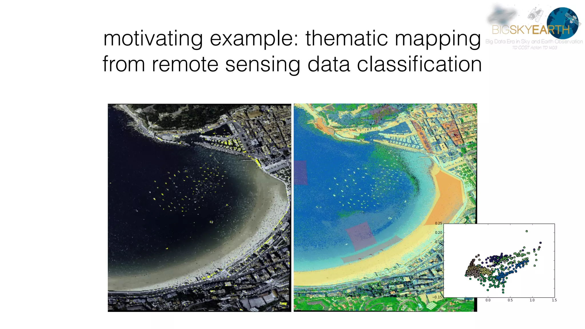
motivating example: thematic mapping   from remote sensing data classiﬁcation

motivation: global scale near real–time analysis • interactive data exploration   (e.g. iteratively supervised thematic mapping) • advanced algorithms for end–user “apps” • e.g. • astronomy “catalogues” • geo analysis tools a la Google EarthEngine

motivation: global scale near real–time analysis • growing remote sensing archive size - volume, variety, velocity • e.g. the Copernicus Sentinels • growing competence palette needed • e.g. forestry, remote sensing, statistics,   computer science, visualisation, operations

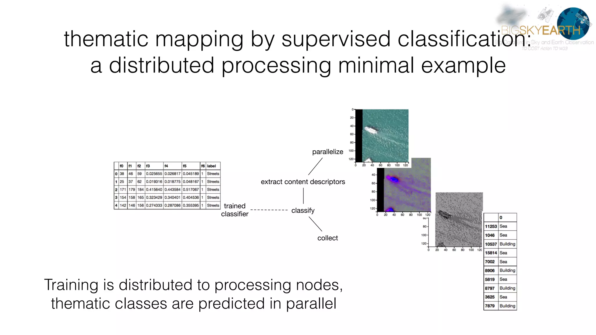
thematic mapping by supervised classiﬁcation: a distributed processing minimal example parallelize extract content descriptors classify trained classiﬁer collect Training is distributed to processing nodes, thematic classes are predicted in parallel

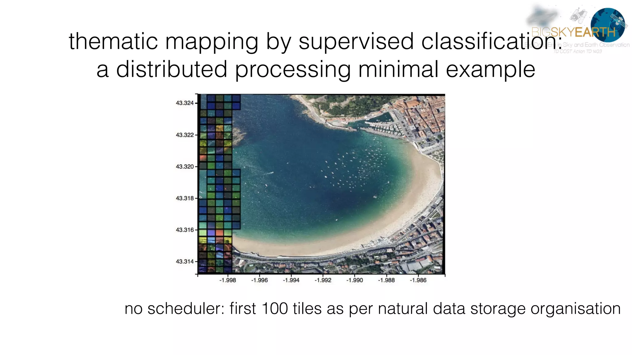
no scheduler: ﬁrst 100 tiles as per natural data storage organisation thematic mapping by supervised classiﬁcation: a distributed processing minimal example

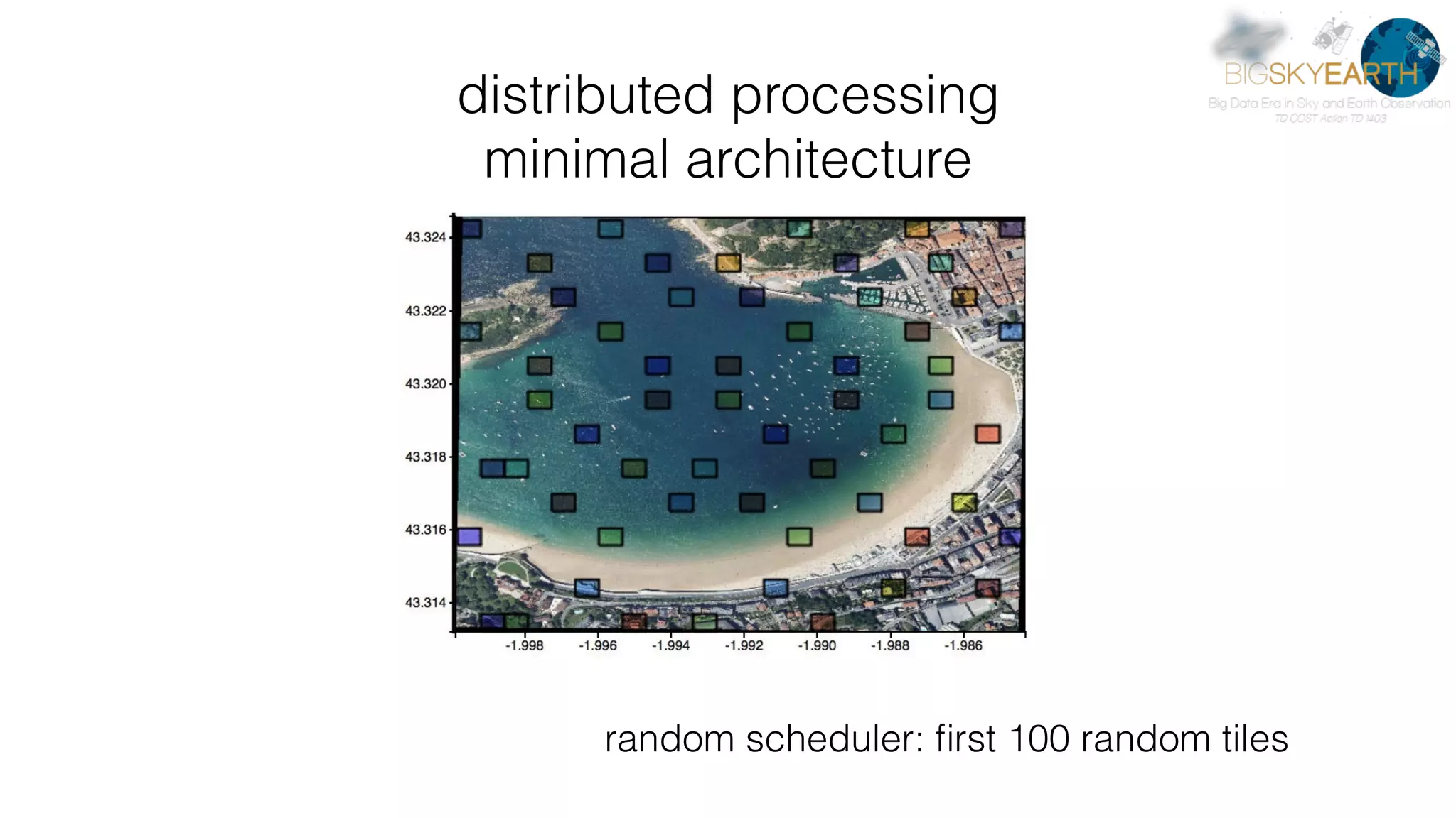
distributed processing  minimal architecture random scheduler: ﬁrst 100 random tiles

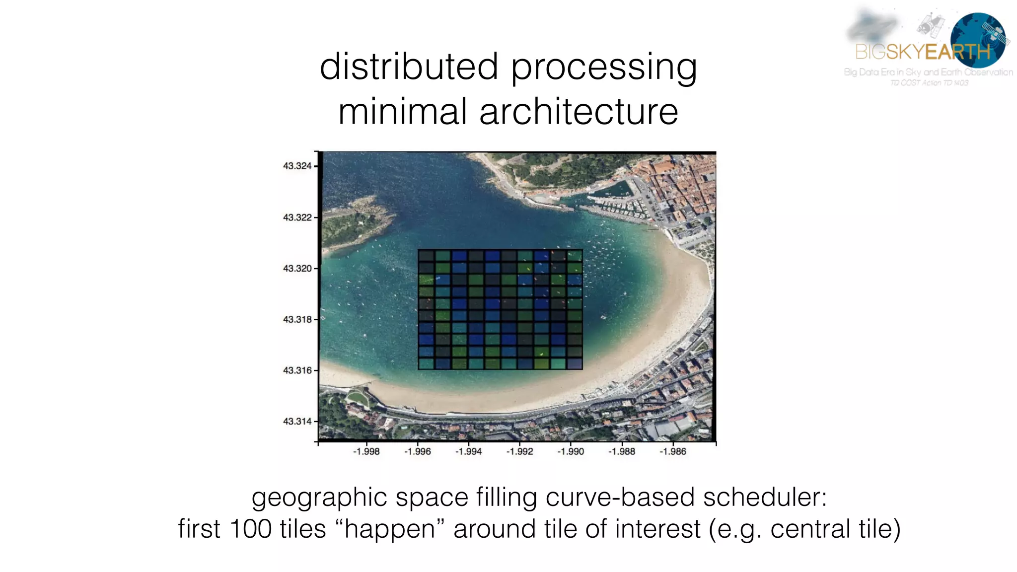
distributed processing  minimal architecture geographic space ﬁlling curve-based scheduler:   ﬁrst 100 tiles “happen” around tile of interest (e.g. central tile)

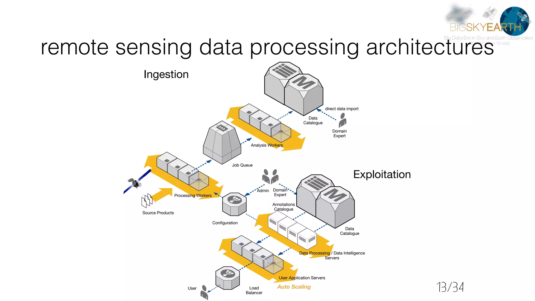
remote sensing data processing architectures Job Queue Analysis Workers Data Catalogue Processing Workers Auto Scaling Ingestion Data Catalogue Exploitation Annotations Catalogue User Application Servers Load Balancer User Source Products Domain Expert Conﬁguration Admin Domain Expert direct data import Data Processing / Data Intelligence Servers 13/34

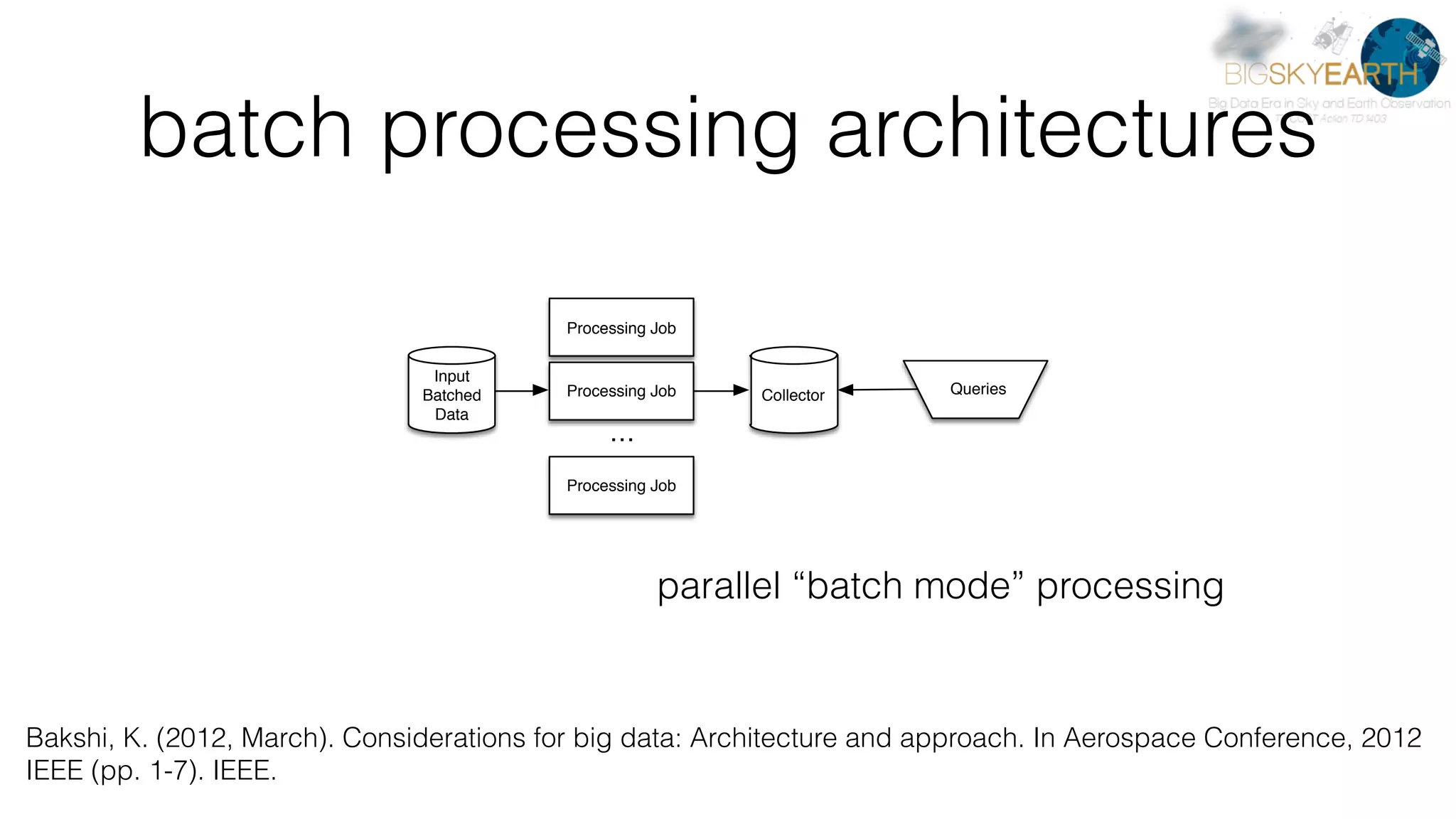
batch processing architectures parallel “batch mode” processing Input Batched Data Collector Processing Job Processing Job Processing Job … Queries Bakshi, K. (2012, March). Considerations for big data: Architecture and approach. In Aerospace Conference, 2012 IEEE (pp. 1-7). IEEE.

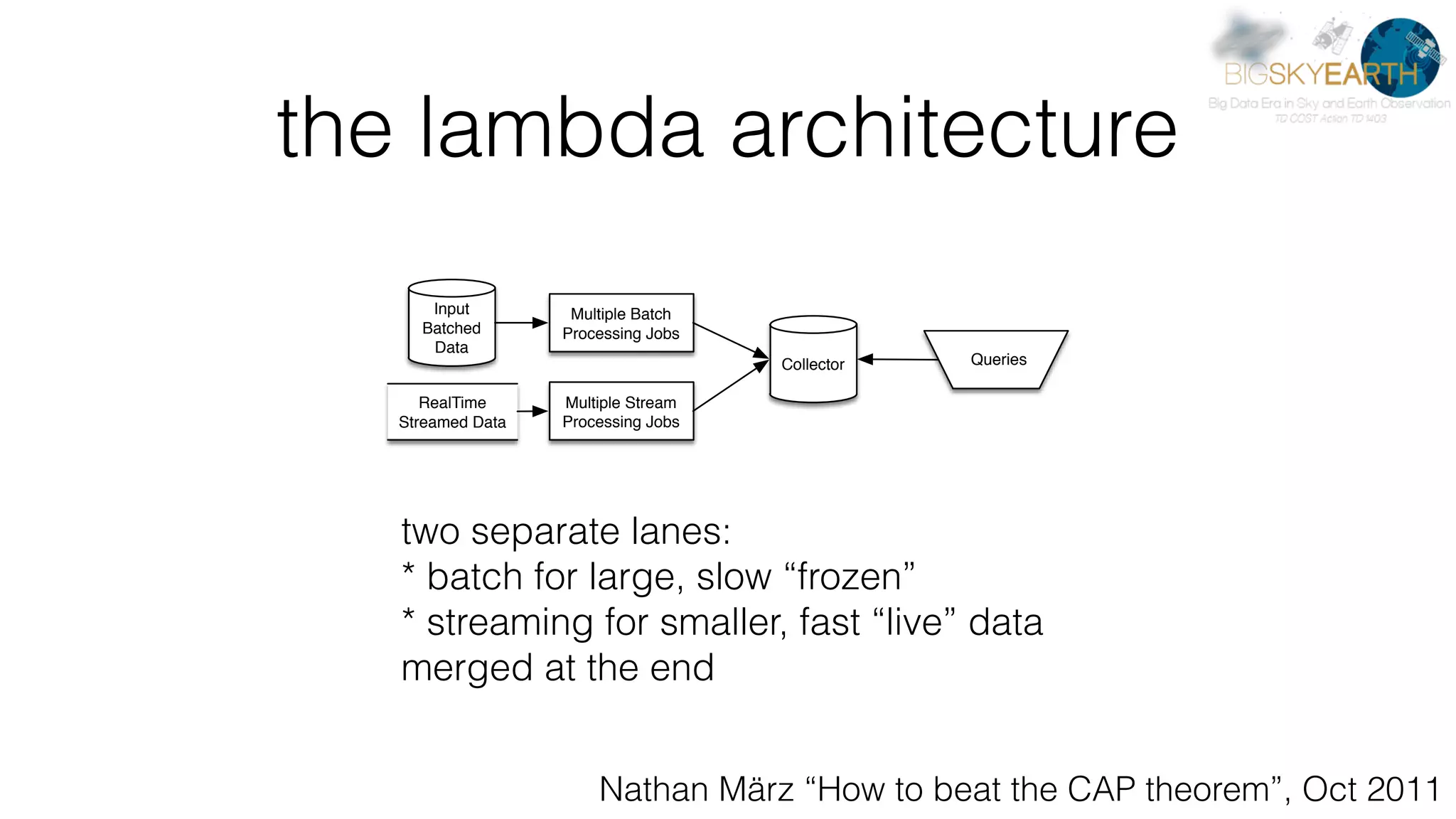
the lambda architecture Nathan März “How to beat the CAP theorem”, Oct 2011 two separate lanes:  * batch for large, slow “frozen”   * streaming for smaller, fast “live” data merged at the end Input Batched Data Collector Multiple Batch Processing Jobs Queries Multiple Stream Processing Jobs RealTime Streamed Data

trade–off considerations • advantages: adaptability  “best of both worlds” –  mixing systems designed with different trade–offs • limits: costs — code maintenance in particular  manifestations of polyglot processing

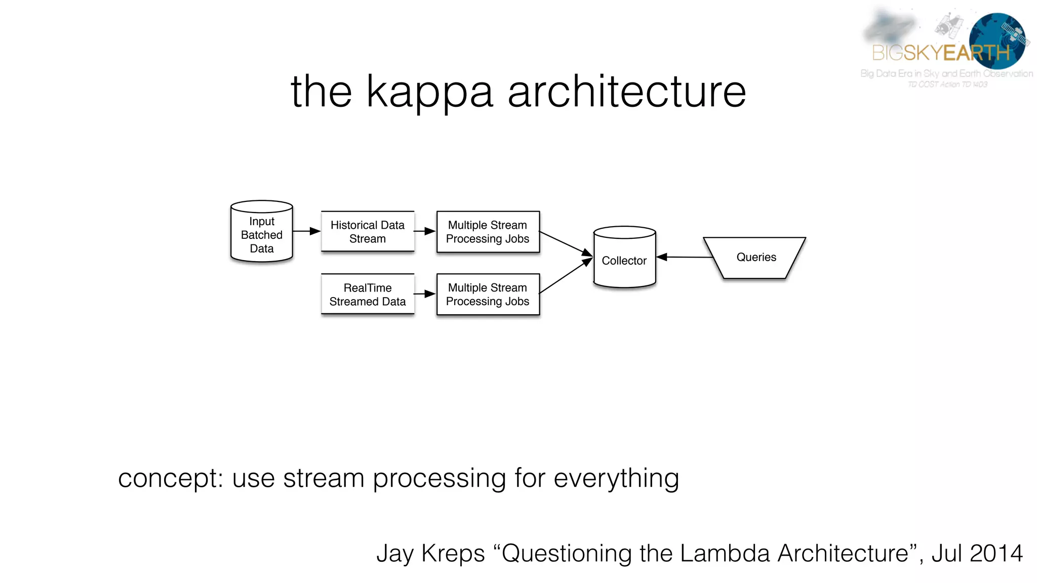
the kappa architecture Jay Kreps “Questioning the Lambda Architecture”, Jul 2014 concept: use stream processing for everything Collector Multiple Stream Processing Jobs Queries Multiple Stream Processing Jobs RealTime Streamed Data Historical Data Stream Input Batched Data

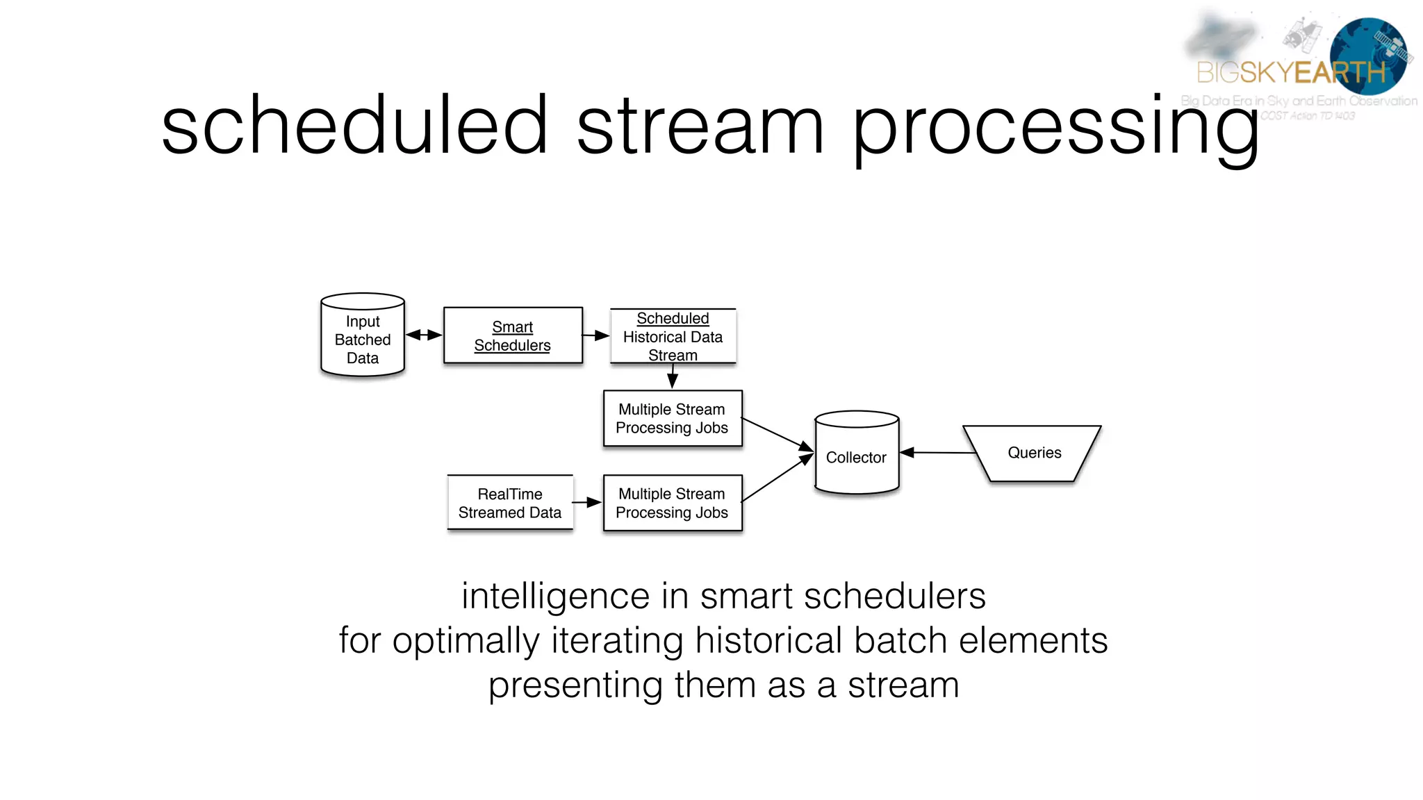
scheduled stream processing intelligence in smart schedulers  for optimally iterating historical batch elements  presenting them as a stream Collector Multiple Stream Processing Jobs Queries Multiple Stream Processing Jobs RealTime Streamed Data Scheduled Historical Data Stream Input Batched Data Smart Schedulers

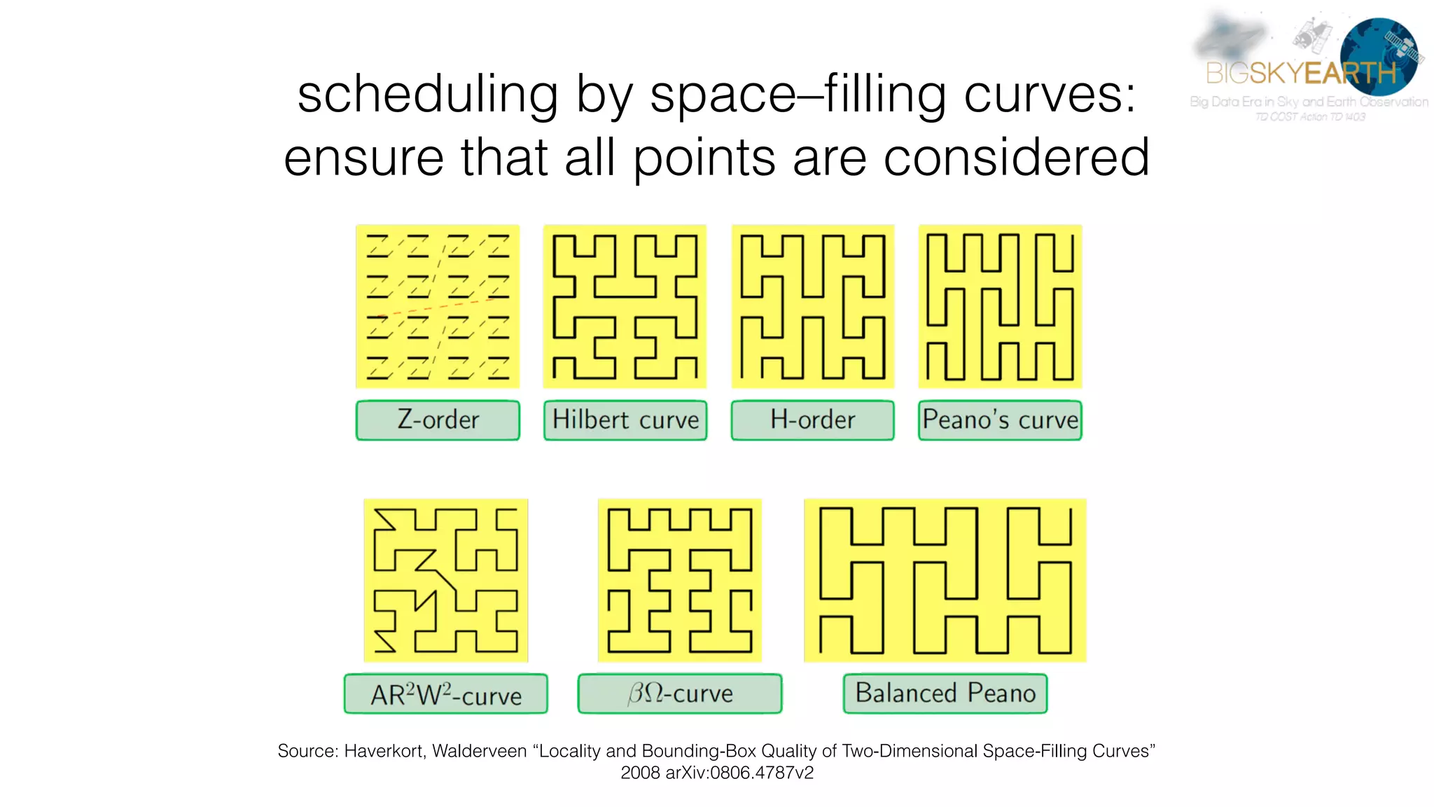
scheduling by space–ﬁlling curves:  ensure that all points are considered Source: Haverkort, Walderveen “Locality and Bounding-Box Quality of Two-Dimensional Space-Filling Curves”   2008 arXiv:0806.4787v2

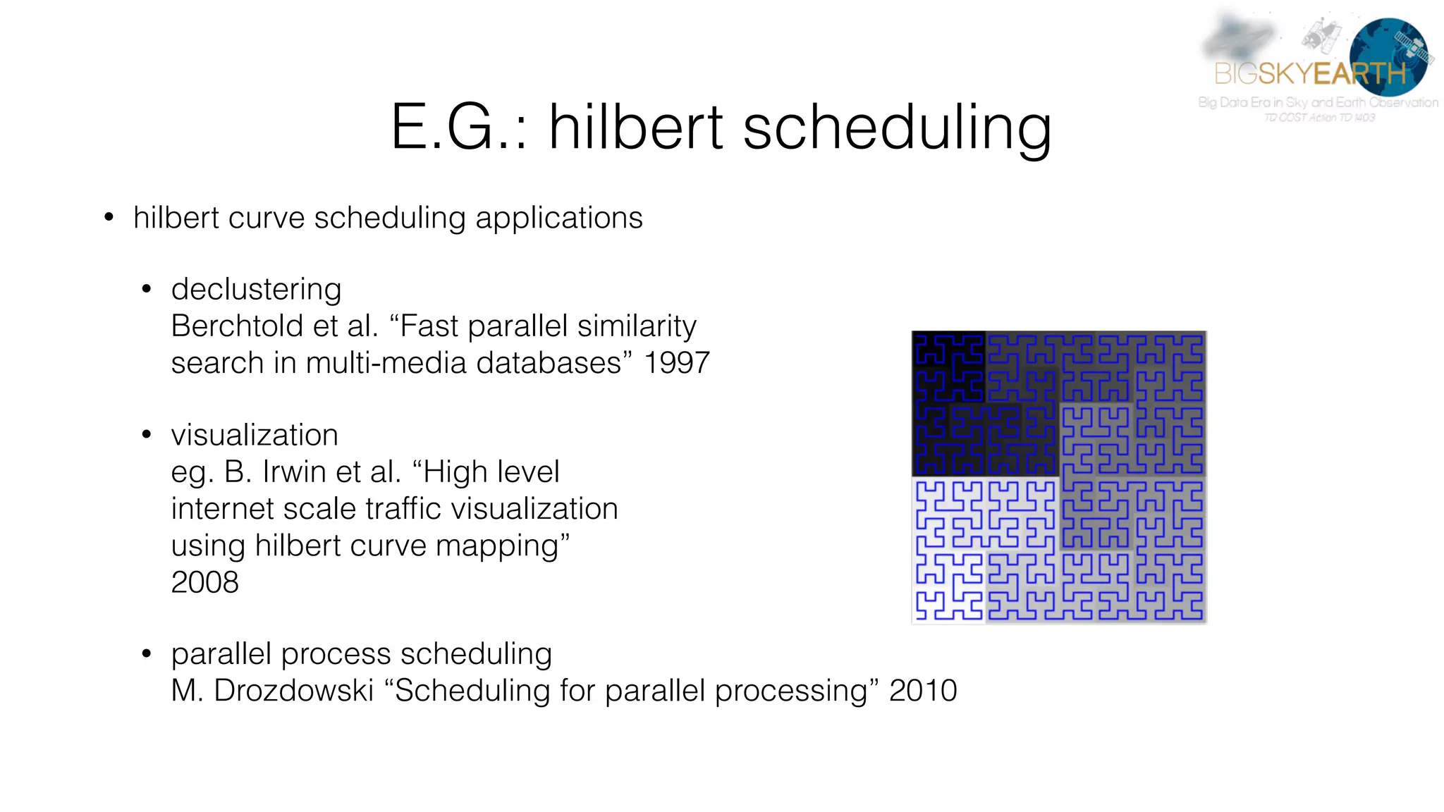
E.G.: hilbert scheduling • hilbert curve scheduling applications • declustering  Berchtold et al. “Fast parallel similarity   search in multi-media databases” 1997 • visualization  eg. B. Irwin et al. “High level   internet scale trafﬁc visualization   using hilbert curve mapping”  2008 • parallel process scheduling  M. Drozdowski “Scheduling for parallel processing” 2010

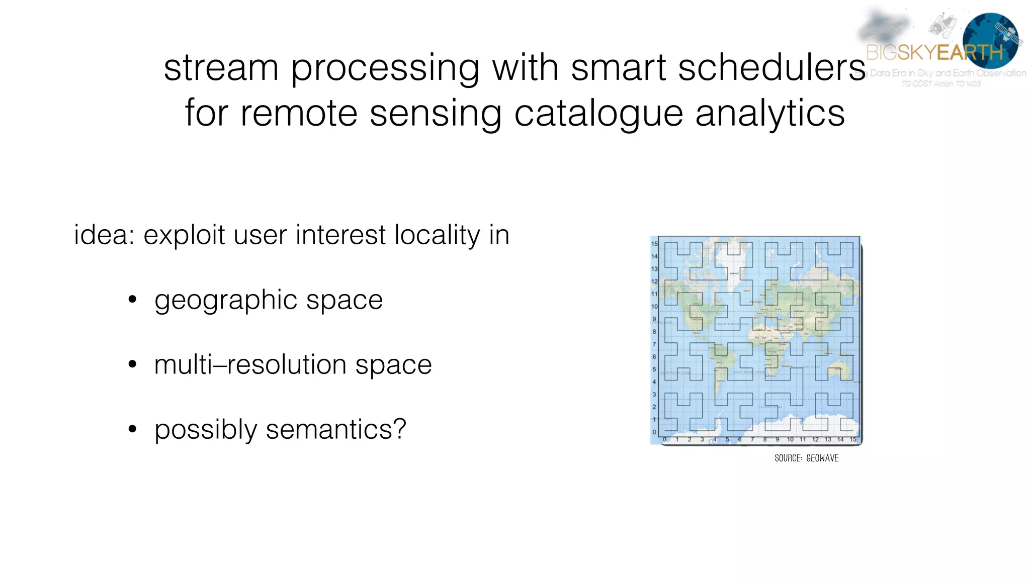
stream processing with smart schedulers   for remote sensing catalogue analytics idea: exploit user interest locality in • geographic space • multi–resolution space • possibly semantics? source: geowave

for large datasets: divide and conquer yet: 1. dependencies need to be modelled (e.g. segmentation) 2. if NOT ALL TILES HAVE EQUAL VALUE  and analysis cost (e.g. TIME) ENTERS THE PICTURE… motivating example: thematic mapping   from remote sensing data classiﬁcation

Part 2: the PyData stack ➤ pydata — data analytics http://pydata.org/downloads/ ➤ rasterio — OO GDAL https://github.com/mapbox/rasterio ➤ fiona — OO OGR http://toblerity.org/fiona/manual.html ➤ skimage — image processing http://scikit-image.org/ ➤ sklearn — machine learning http://scikit-learn.org/stable/ ➤ pandas — data analysis http://pandas.pydata.org/ ➤ PIL — imaging http://www.pythonware.com/products/pil/ ➤ Scipy — scientific computing library http://scipy.org/

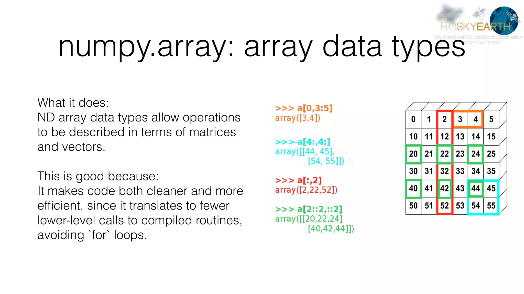
numpy.array: array data types What it does: ND array data types allow operations to be described in terms of matrices and vectors. This is good because: It makes code both cleaner and more efﬁcient, since it translates to fewer lower-level calls to compiled routines, avoiding `for` loops.

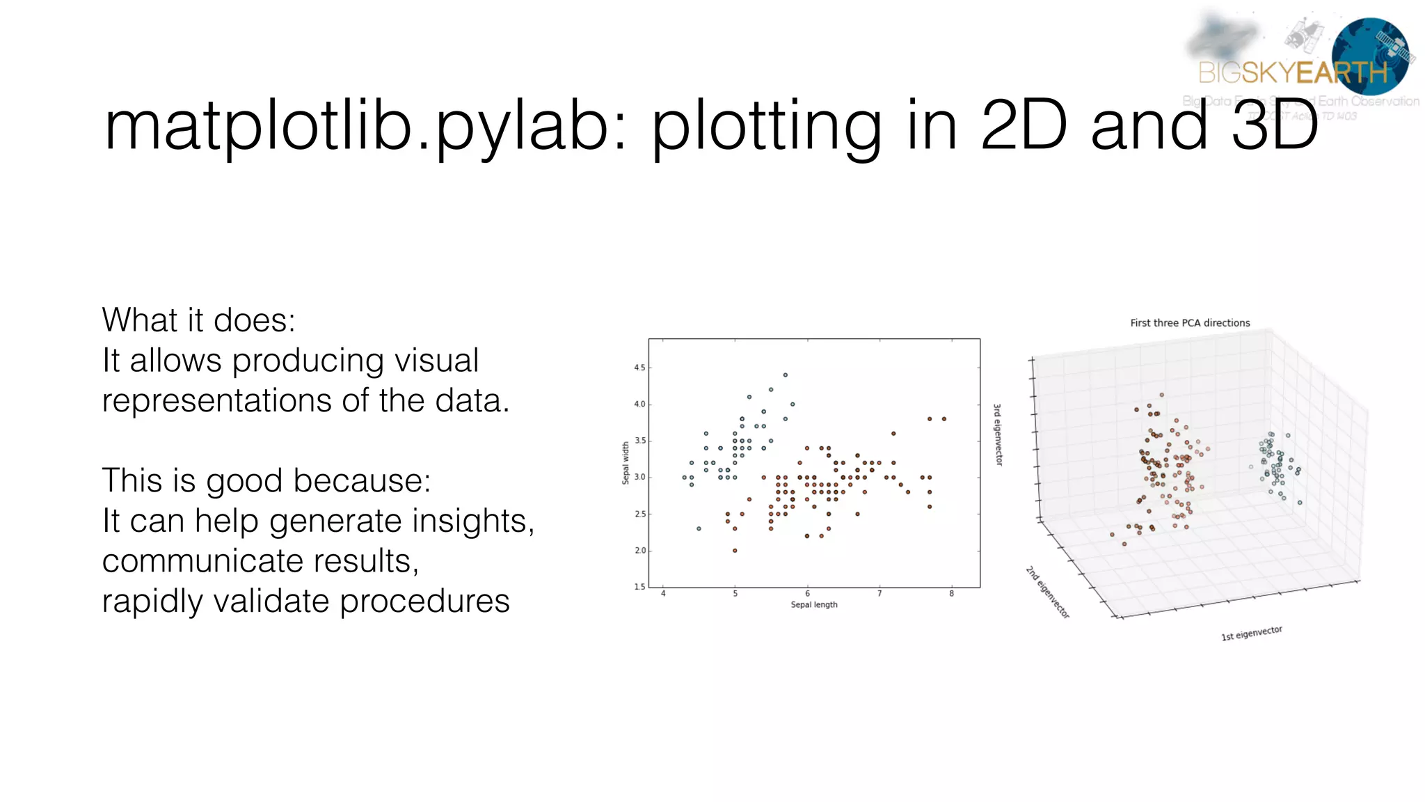
matplotlib.pylab: plotting in 2D and 3D What it does: It allows producing visual representations of the data. This is good because: It can help generate insights, communicate results,   rapidly validate procedures

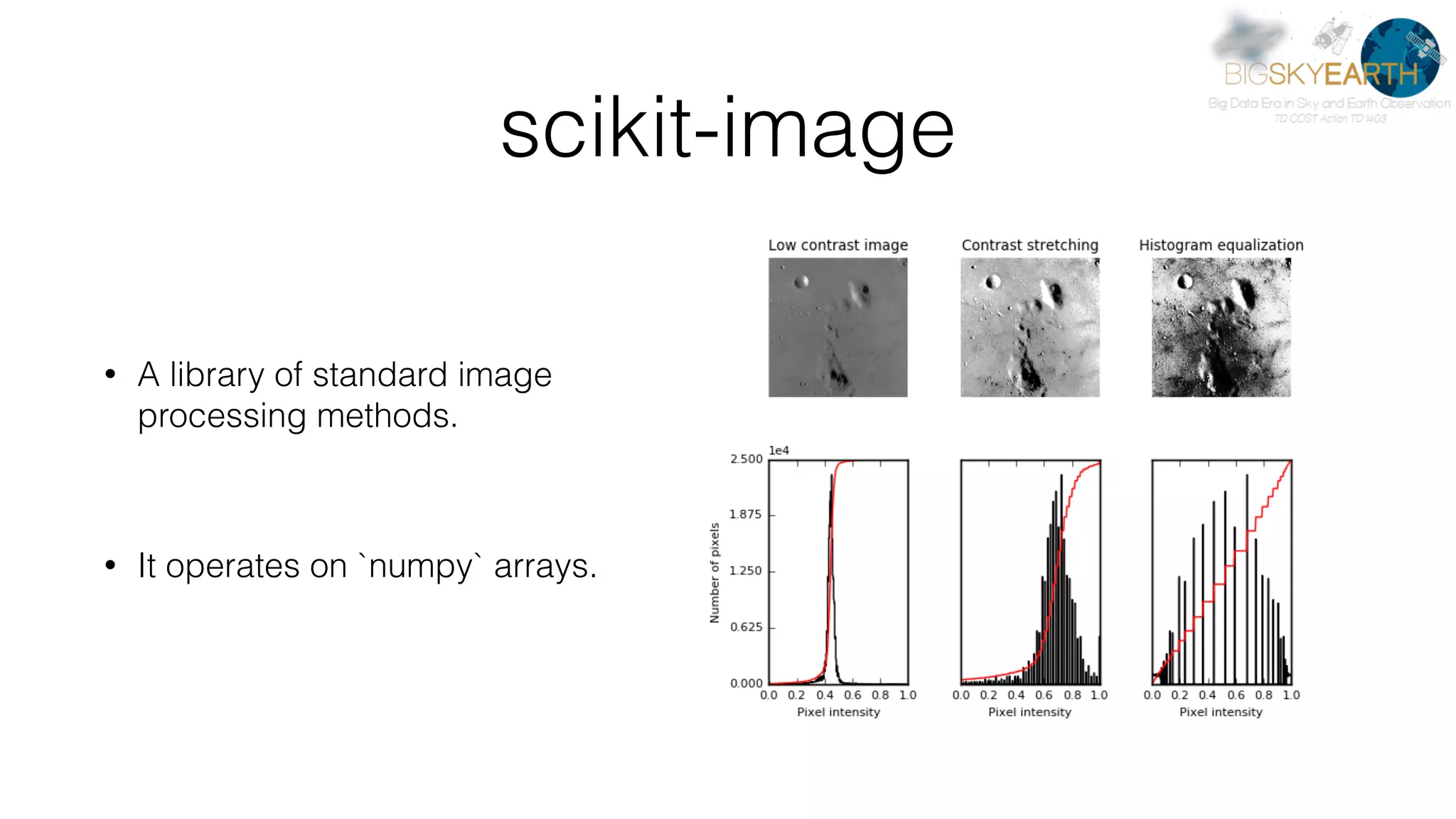
scikit-image • A library of standard image processing methods. • It operates on `numpy` arrays.

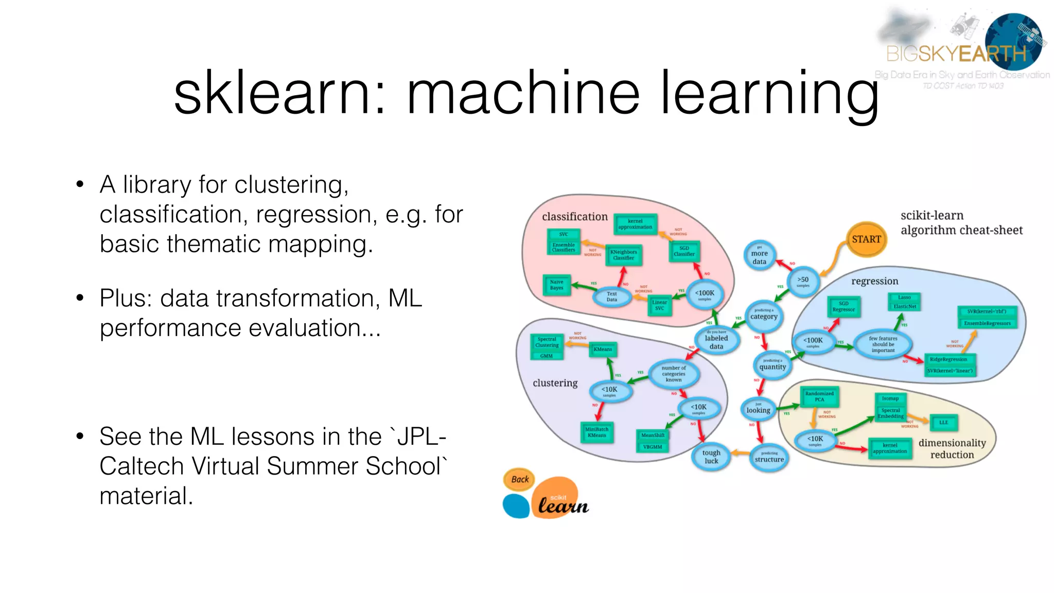
sklearn: machine learning • A library for clustering, classiﬁcation, regression, e.g. for basic thematic mapping. • Plus: data transformation, ML performance evaluation... • See the ML lessons in the `JPL- Caltech Virtual Summer School` material.

RASTERIO: RASTER LOADING ➤ high-level interfaces to GDAL fn = “~/Data/all_donosti_croped_16_wgs4326_b.ers” import rasterio, numpy with rasterio.drivers(CPL_DEBUG=True): with rasterio.open(os.path.expanduser(fn)) as src: bands = map(src.read_band, (1, 2, 3)) data = numpy.dstack(bands) print(type(data)) print(src.bounds) print(src.count, src.shape) print(src.driver) print(str(src.crs)) bounds = src.bounds[::2] + src.bounds[1::2] import skimage.color import matplotlib.pylab as plt data_hsv = skimage.color.rgb2xyz(data) fig = plt.figure(figsize=(8, 8)) ax = plt.imshow(data_hsv, extent=bounds) plt.show()

FIONA: VECTOR MASKING ➤ Binary masking by Shapefiles import shapefile, os.path from PIL import Image, ImageDraw sf = shapefile.Reader(os.path.expanduser(“~/masking_shapes.shp")) shapes, src_bbox = sf.shapes(), [ bounds[i] for i in [0, 2, 1, 3] ] # Geographic x & y image sizes xdist, ydist = src_bbox[2] - src_bbox[0], src_bbox[3] - src_bbox[1] # Image width & height iwidth, iheight = feats.shape[1], feats.shape[0] xratio, yratio = iwidth/xdist, iheight/ydist # Masking mask = Image.new("RGB", (iwidth, iheight), "black") draw = ImageDraw.Draw(mask) pixels = { label:[] for label in labels } for i_shape, shape in enumerate(sf.shapes()): draw.polygon([ p[:2] for p in pixels[label] ], outline="rgb(1, 1, 1)", fill="rgb(1, 1, 1)”) import scipy.misc fig = plt.figure(figsize=(8, 8)) ax = plt.imshow(scipy.misc.fromimage(mask)*data, extent=bounds)

pandas: data management and analysis • Adds labels to `numpy` arrays. • Mimicks R's DataFrame type, integrates plotting and data analysis.

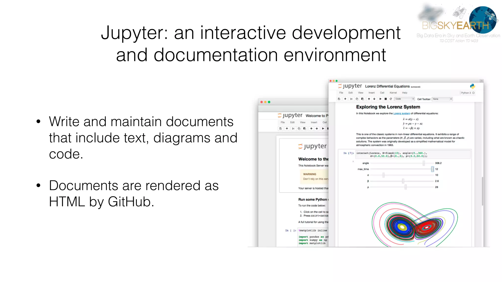
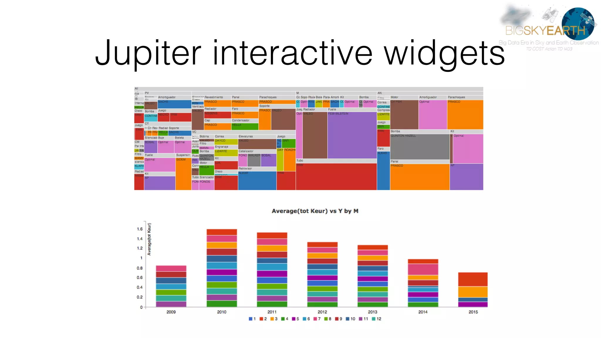
Jupyter: an interactive development   and documentation environment • Write and maintain documents that include text, diagrams and code. • Documents are rendered as HTML by GitHub.

Part 3: Cluster computing • Idea: “Decompose data, move instructions to data chunks” • Big win for easily decomposable problems • Issues in managing dependencies in data analysis

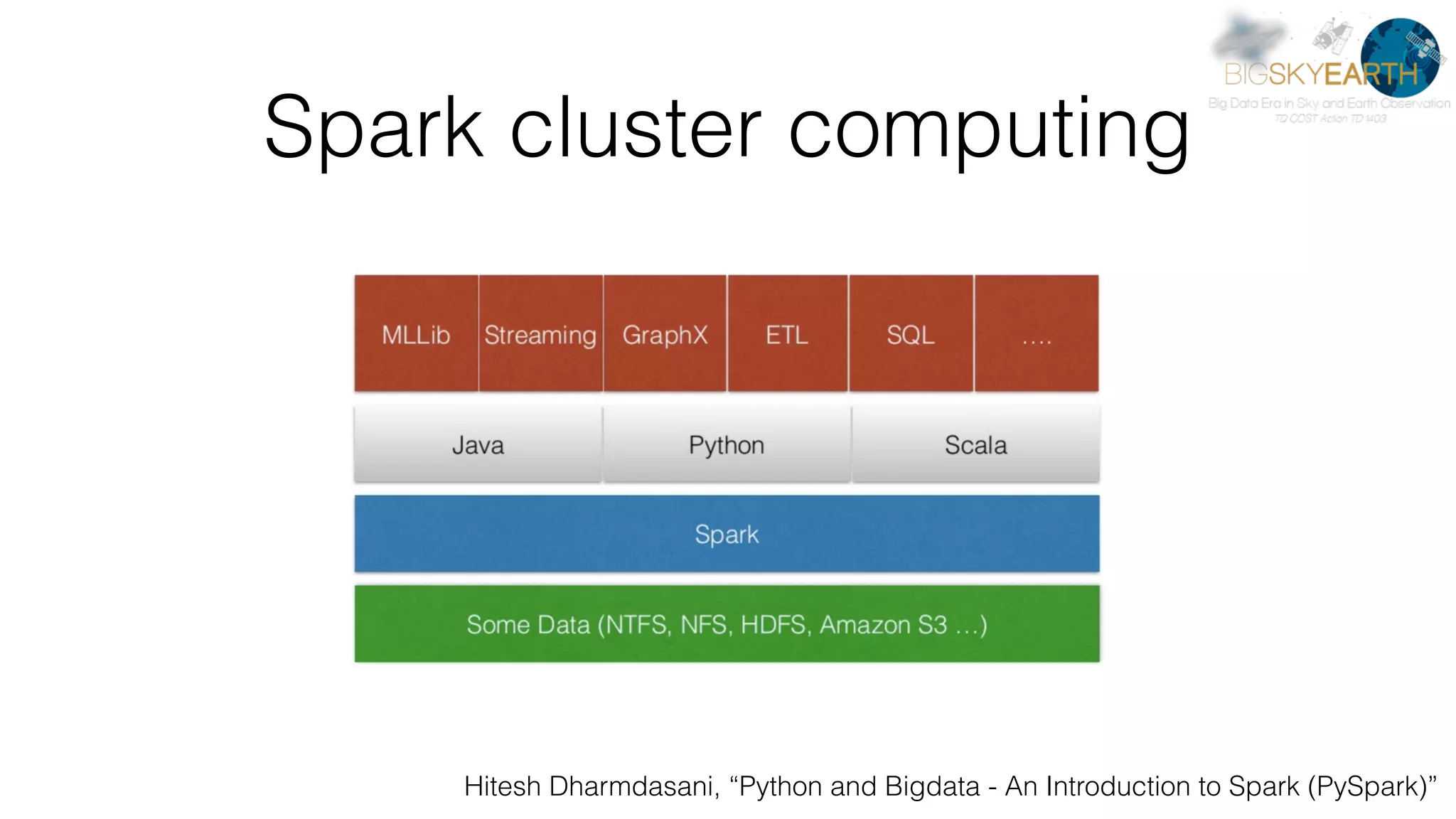
Spark cluster computing Hitesh Dharmdasani, “Python and Bigdata - An Introduction to Spark (PySpark)”

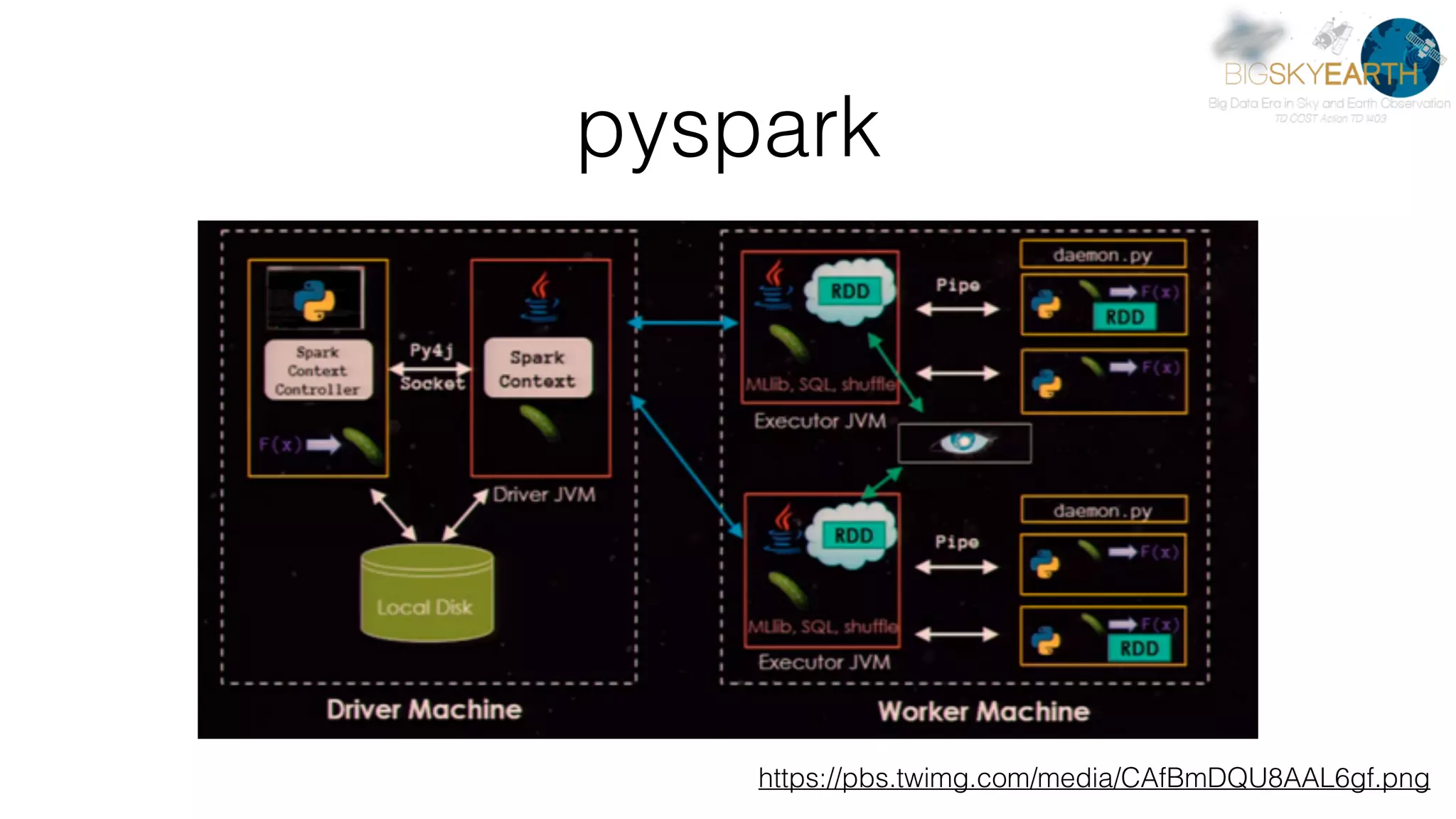
pyspark https://pbs.twimg.com/media/CAfBmDQU8AAL6gf.png

pyspark example: context The Spark context represents the cluster. It can be used to distribute elements to the nodes. Examples: - a library module - a query description in a search system.

pyspark example: hdfs Distributes and manages for redundancy very large data ﬁles on the cluster disks. Achille's heel: managing very large numbers of small ﬁles.

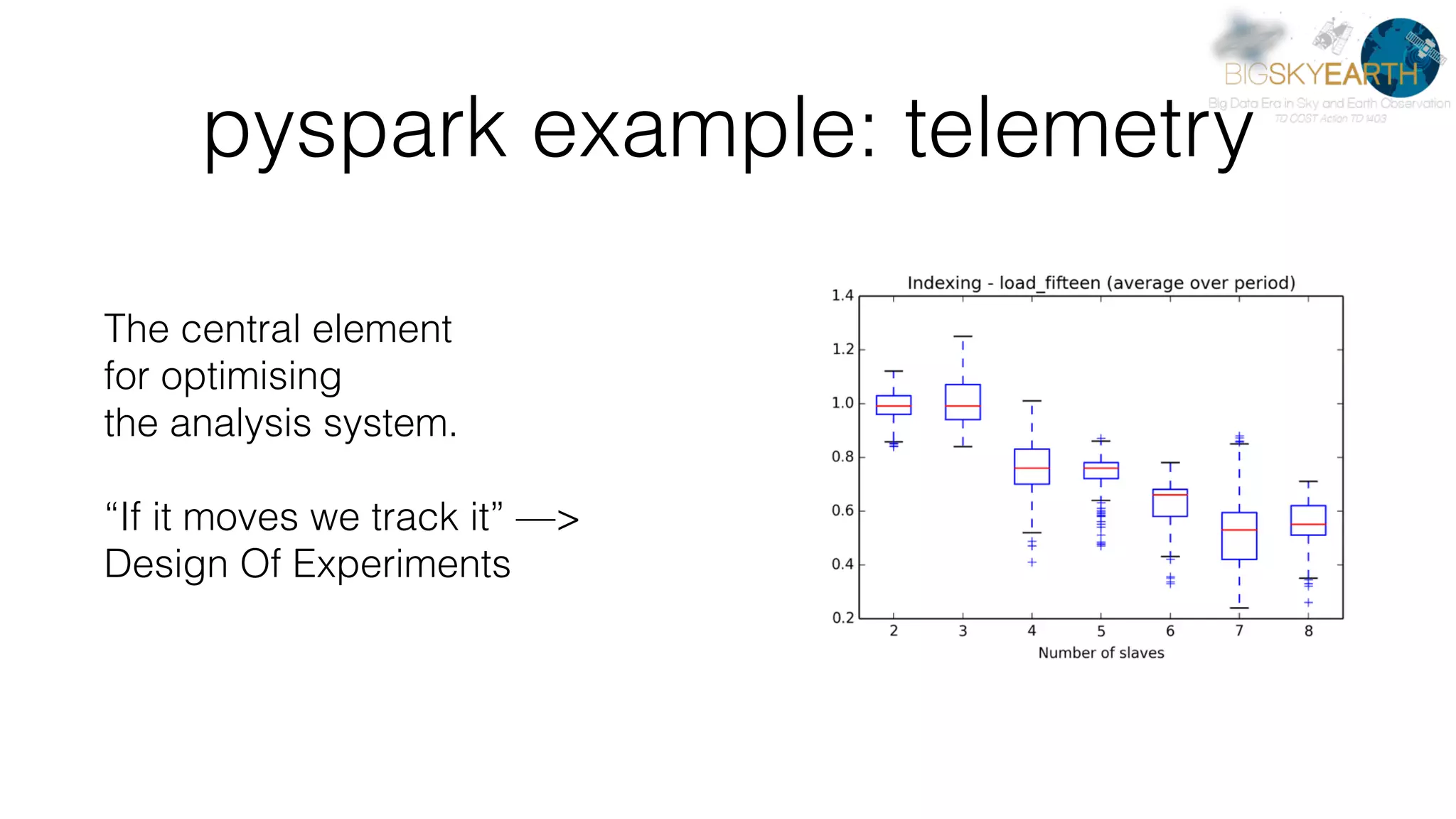
pyspark example: telemetry The central element for optimising the analysis system. “If it moves we track it” —> Design Of Experiments

pyspark example: spark.mllib Machine learning tools for cluster computing contexts   is a central application of cluster computing frameworks.  At times, still not up to par with single machine conﬁgurations.

pyspark.streaming Data stream analysis (e.g. from a network connection) an important use case. Standard cluster computing concepts apply. It is done in chunks whose size is not controlled directly.

pyspark @ AWS The Spark distribution includes tools to instantiate a cluster on the Amazon Web Services infrastructure. Costs tend to be extremely low…  if you DO NOT publish your credentials.

Ongoing trends • Data standardisation: Apache Arrow • A simpliﬁcation of infrastructure management tools: Hashi Terraform

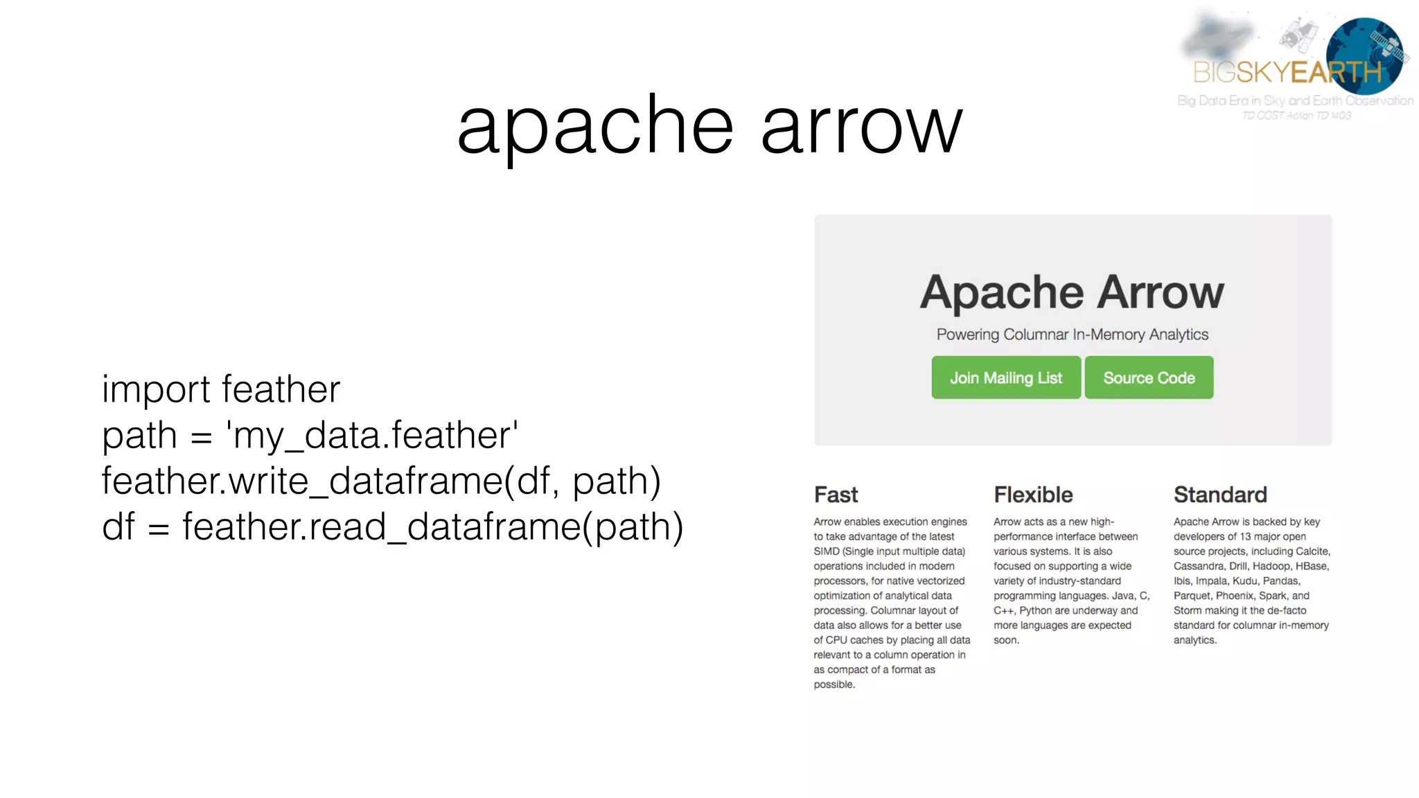
apache arrow import feather path = 'my_data.feather' feather.write_dataframe(df, path) df = feather.read_dataframe(path)

OpenStack, Ansible, Vagrant, Terraform... • Infrastructure management tools   allow more complex setups to be easily managed

Conclusions • Extending an analytics pipeline to computing clusters   can be done with limited resources

04 open source_tools

More Related Content

What's hot

Viewers also liked

Similar to 04 open source_tools

Recently uploaded

04 open source_tools