Automated Data Exploration Building efficient analysis pipelines with Dask Víctor Zabalza victor.z@asidatascience.com @zblz @ASIDataScience
About me • Data engineer at ASI Data Science. • Former astrophysicist. • Main developer of naima, a Python package for radiative analysis of non-thermal astronomical sources. • matplotlib developer.
ASI Data Science • Data science consultancy • Academia to Data Industry fellowship • SherlockML
Data Exploration
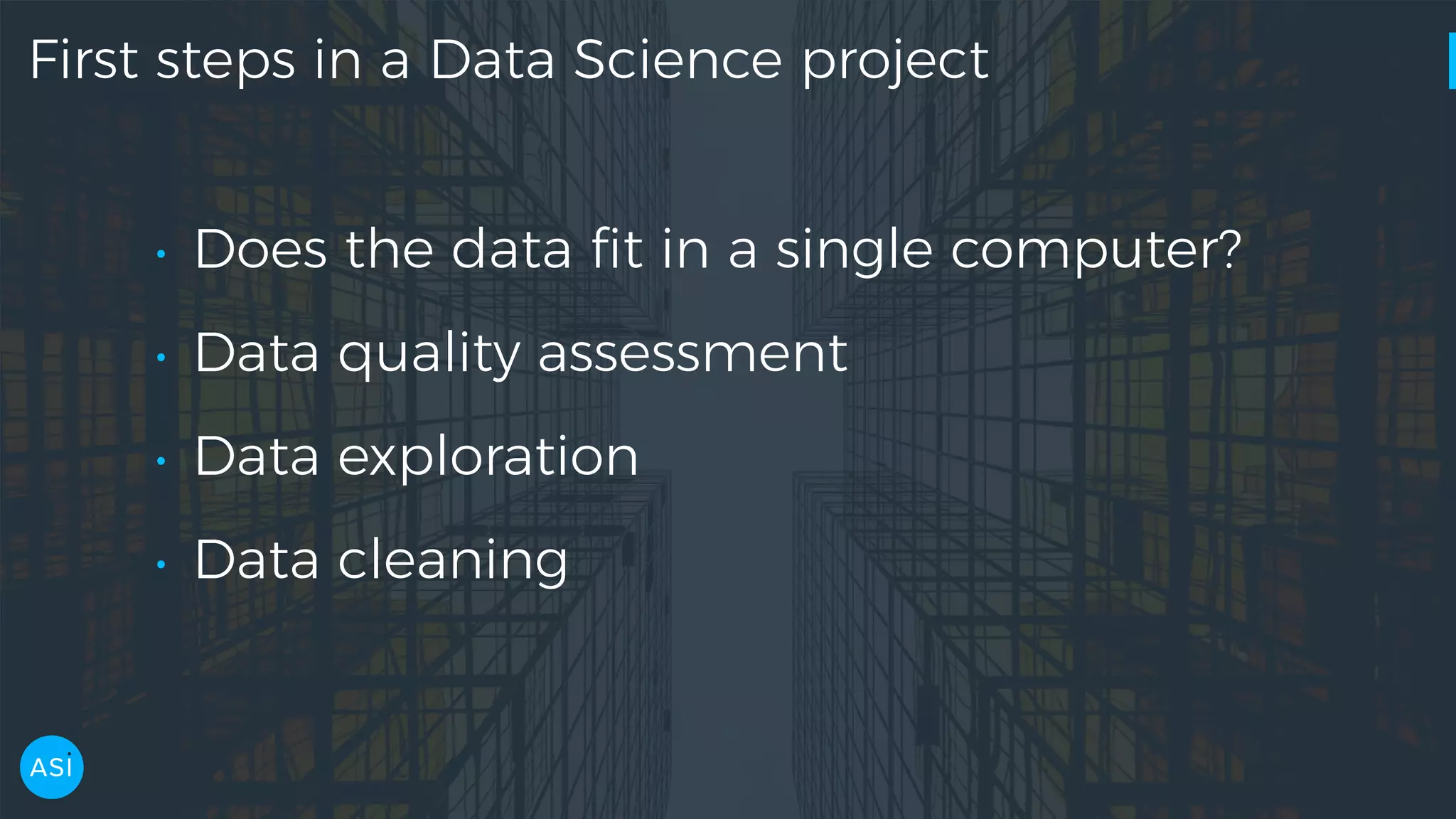
First steps in a Data Science project • Does the data fit in a single computer? • Data quality assessment • Data exploration • Data cleaning
80% → >30 h/week
Can we automate the drudge work?
Developing a tool for data exploration based on Dask
Lens Library and service for automated data quality assessment and exploration
Lens by example Room occupancy dataset • ML standard dataset • Goal: predict occupancy based on ambient measurements. • What can we learn about it with Lens?
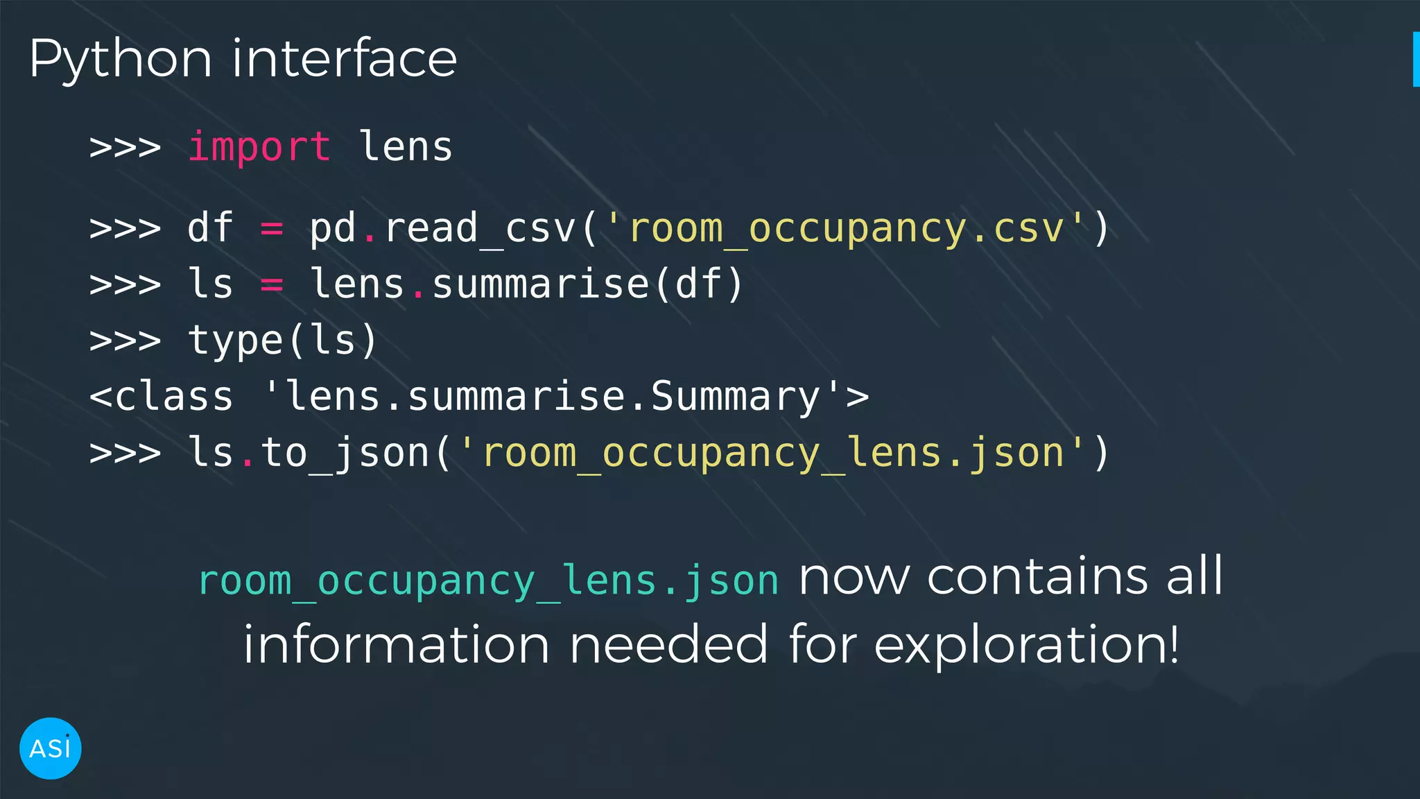
Python interface >>> import lens >>> df = pd.read_csv('room_occupancy.csv') >>> ls = lens.summarise(df) >>> type(ls) <class 'lens.summarise.Summary'> >>> ls.to_json('room_occupancy_lens.json') room_occupancy_lens.json now contains all information needed for exploration!
Python interface — Columns >>> ls = lens.Summary.from_json('room_occupancy_lens.json') >>> ls.columns ['date', 'Temperature', 'Humidity', 'Light', 'CO2', 'HumidityRatio', 'Occupancy']
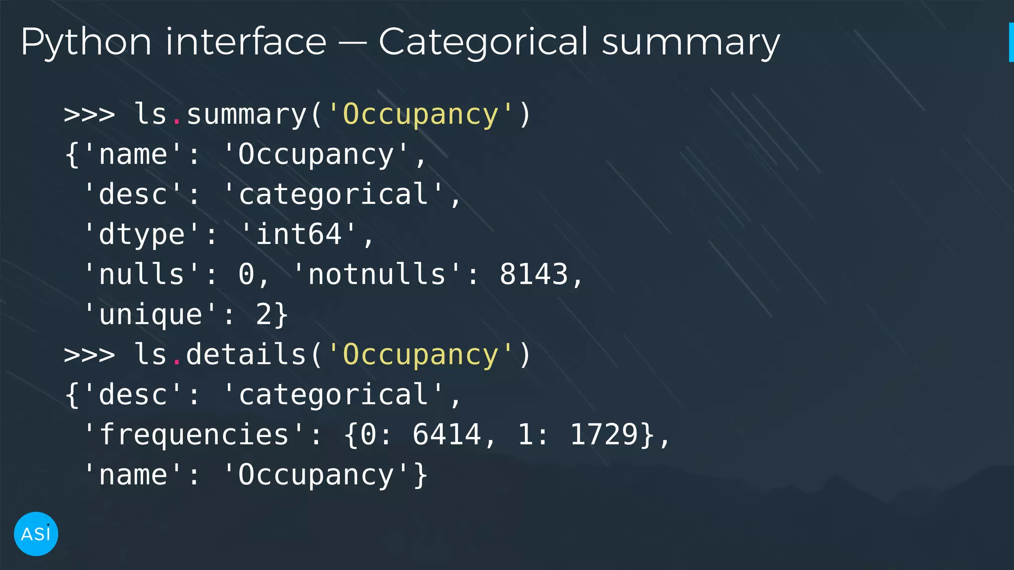
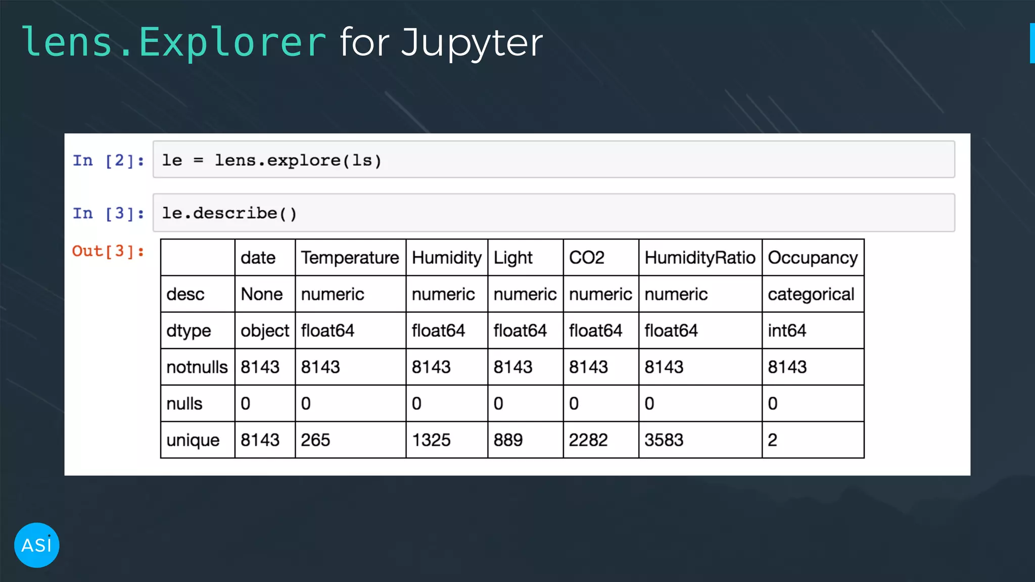
Python interface — Categorical summary >>> ls.summary('Occupancy') {'name': 'Occupancy', 'desc': 'categorical', 'dtype': 'int64', 'nulls': 0, 'notnulls': 8143, 'unique': 2} >>> ls.details('Occupancy') {'desc': 'categorical', 'frequencies': {0: 6414, 1: 1729}, 'name': 'Occupancy'}
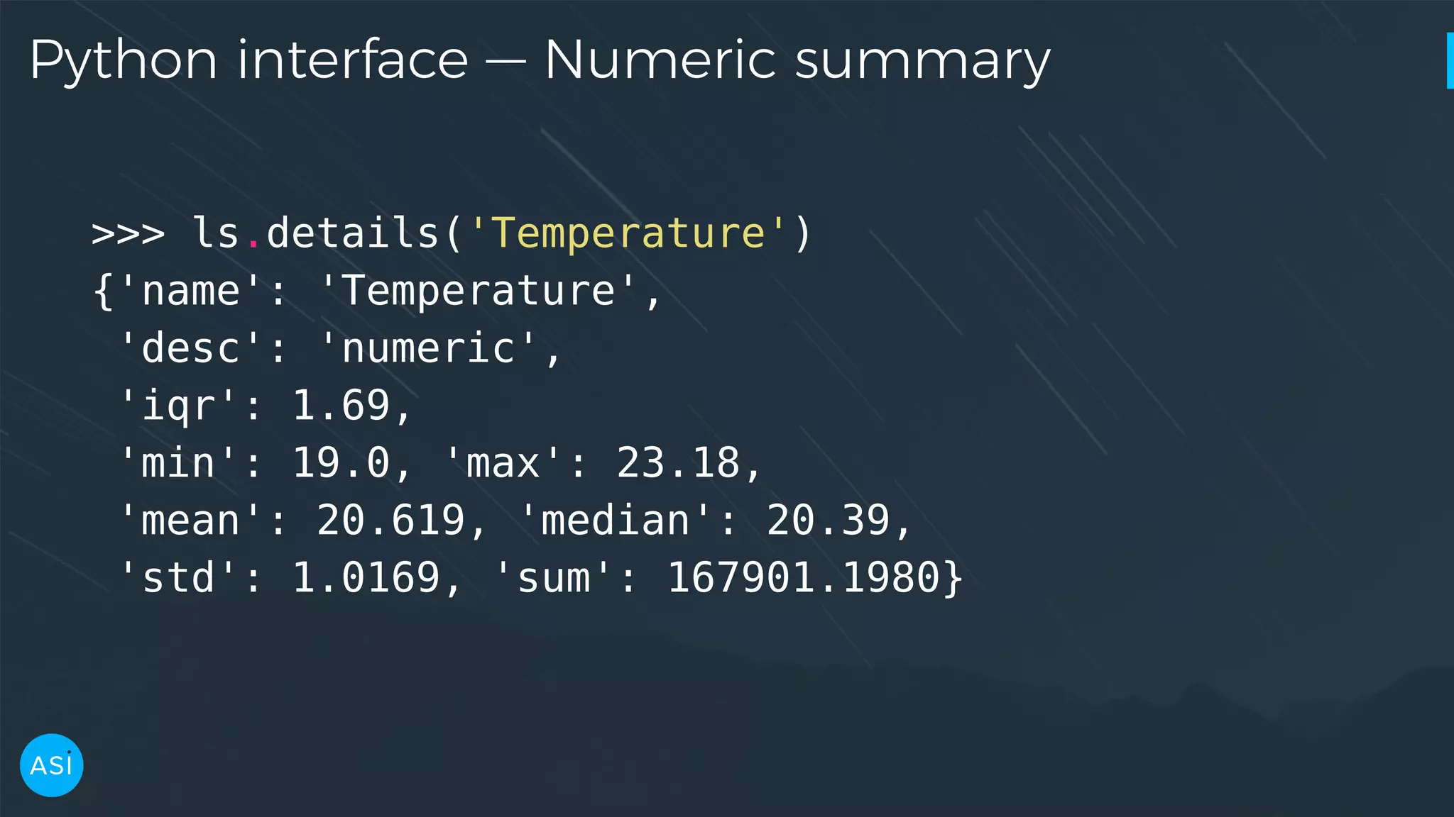
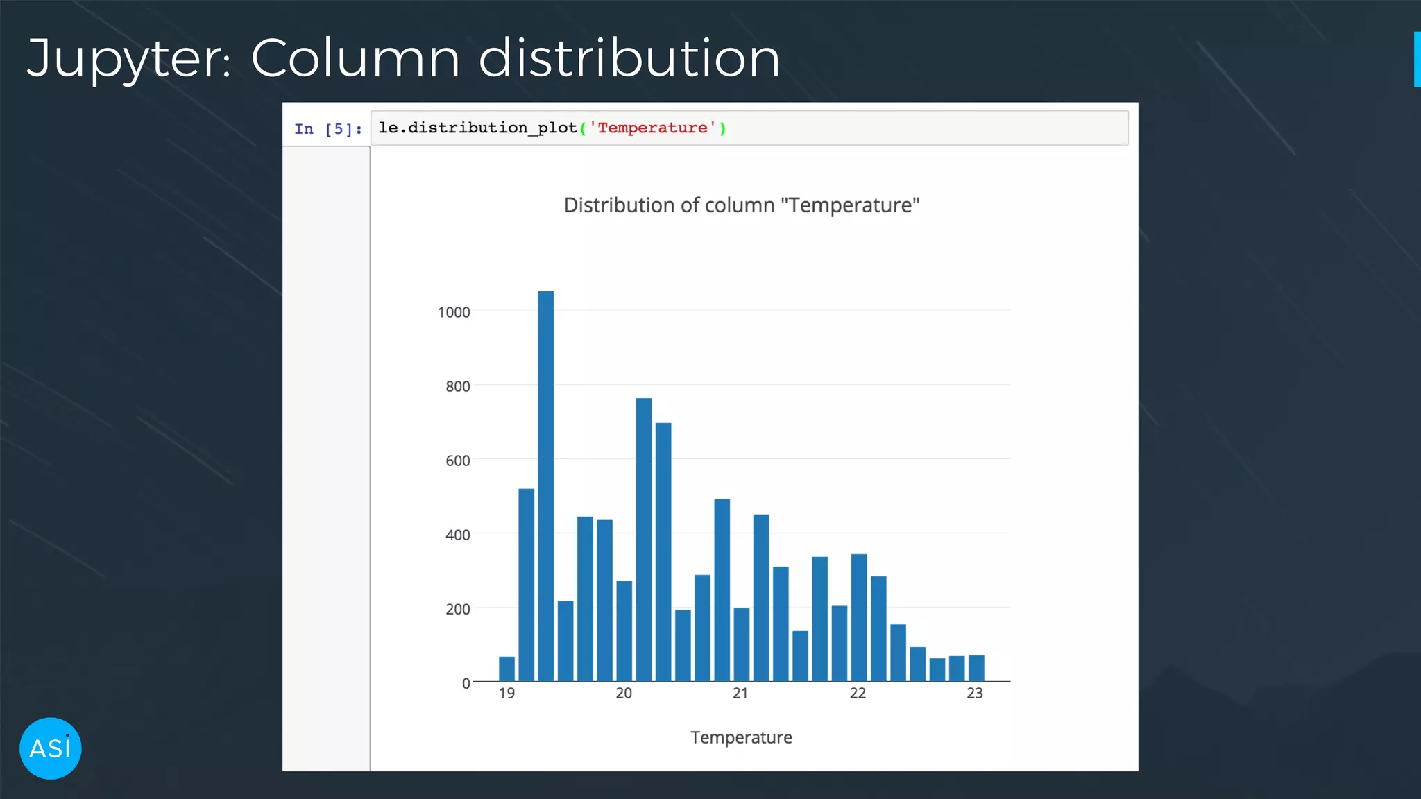
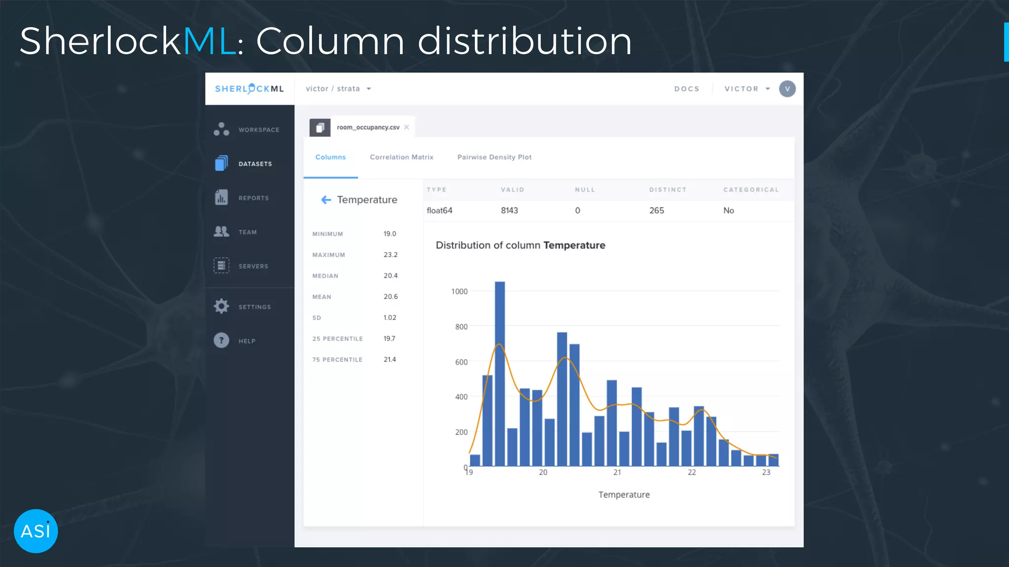
Python interface — Numeric summary >>> ls.details('Temperature') {'name': 'Temperature', 'desc': 'numeric', 'iqr': 1.69, 'min': 19.0, 'max': 23.18, 'mean': 20.619, 'median': 20.39, 'std': 1.0169, 'sum': 167901.1980}
Python interface — KDE, PDF >>> x, y = ls.kde('Temperature') >>> x[np.argmax(y)] 19.417999999999999 >>> temperature_pdf = ls.pdf('Temperature') >>> temperature_pdf([19, 20, 21, 22]) array([ 0.01754398, 0.76491742, 0.58947765, 0.28421244])
The lens.Summary is a good building block, but clunky for exploration. Can we do better?
Jupyter
lens.Explorer for Jupyter
Jupyter: Column distribution
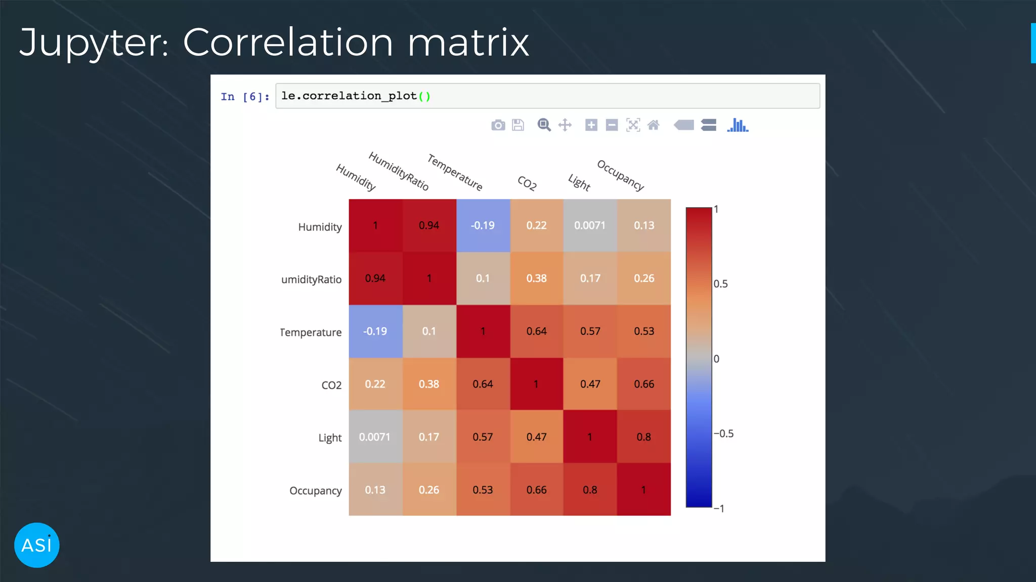
Jupyter: Correlation matrix
Jupyter widgets
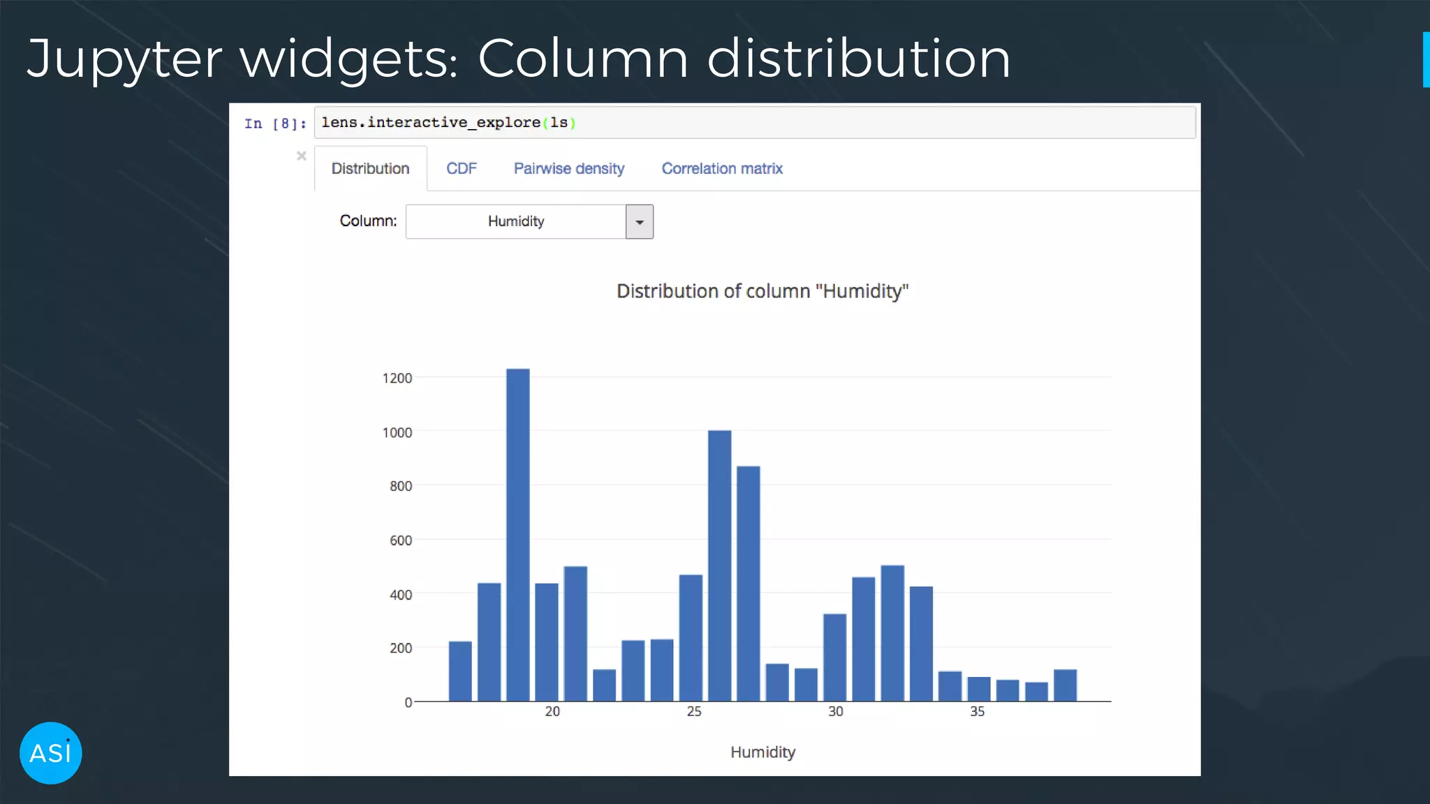
Jupyter widgets: Column distribution
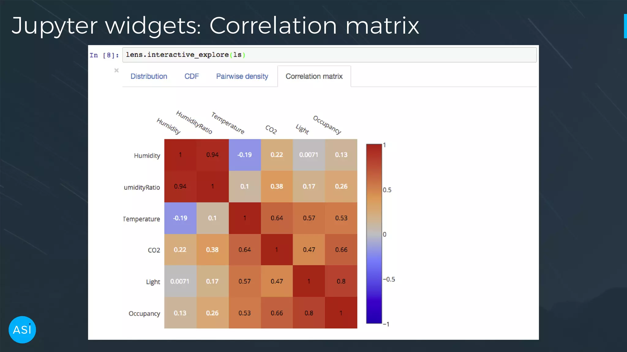
Jupyter widgets: Correlation matrix
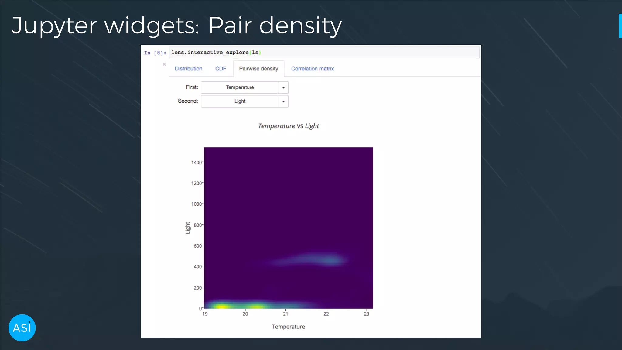
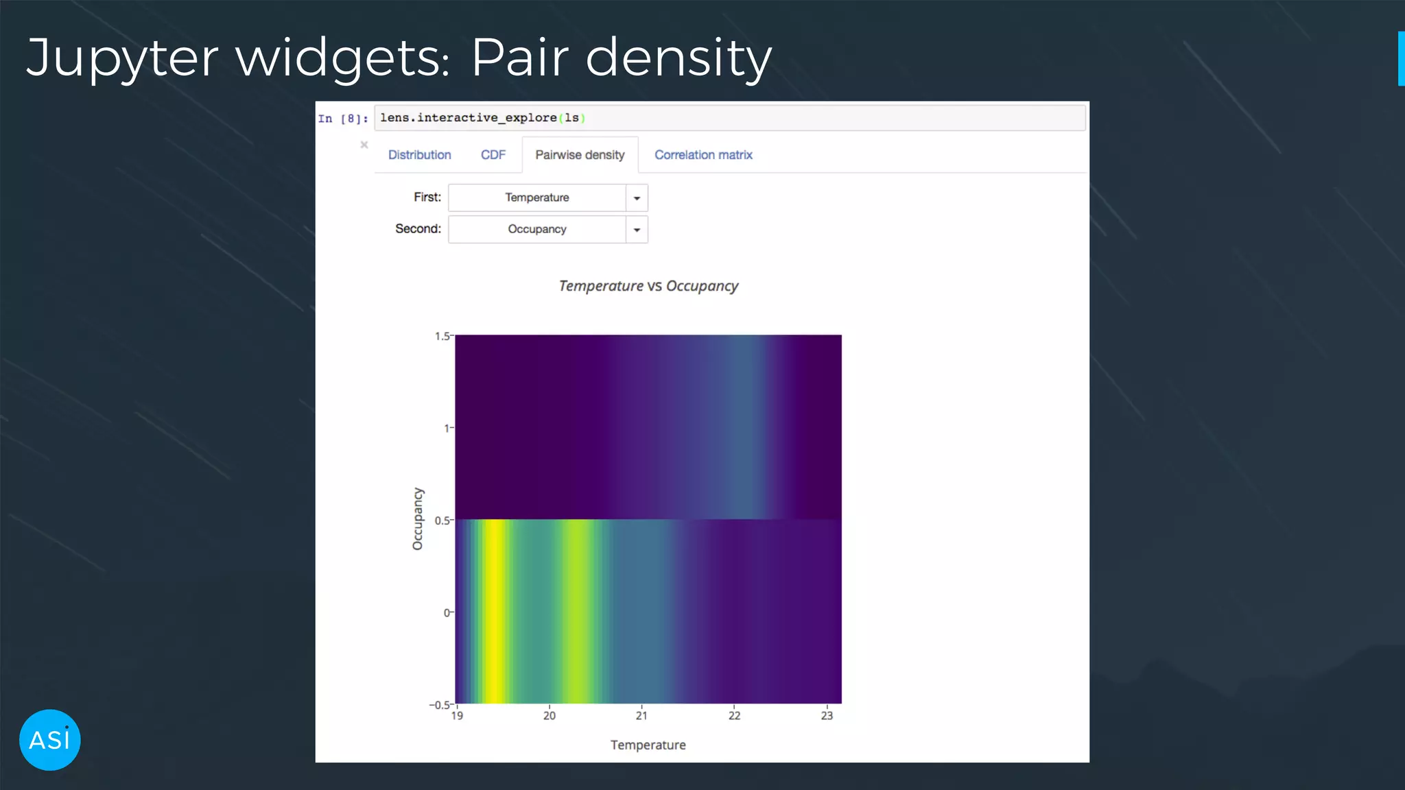
Jupyter widgets: Pair density
Building Lens
Requirements • Versatile • Reproducible • Portable • Scalable • Reusable
Our solution: Analysis • A Python library computes dataset metrics: • Column-wise statistics • Pairwise densities • ... • Computation cost is paid up front. • The result is serialized to JSON.
Our Solution: Interactive exploration • Using only the report, the user can explore the dataset through either: • Jupyter widgets • Web UI
The lens Python library
Why Python? Portability A Python library easily runs in: • Jupyter notebooks for interactive analysis. • One-off scripts. • Scheduled or on-demand jobs in cluster.
Why Python? Reusability • Allows us to use the Python data ecosystem. • Becomes a building block in the Data Science process.
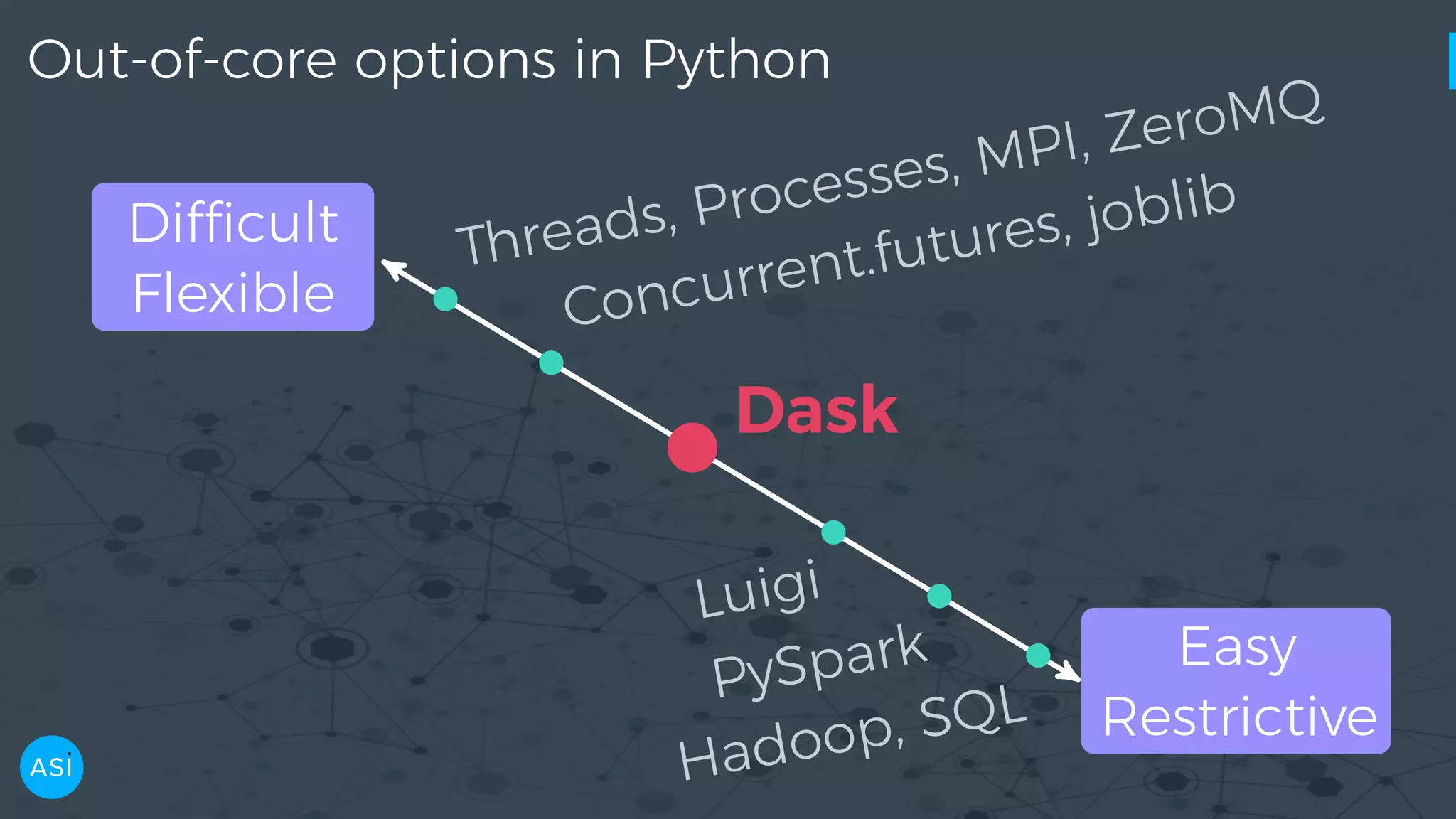
Why Python? Scalability • Python is great for single-core, in-memory, numerical computations through numpy, scipy, pandas. • But the GIL limits its ability to parallelise workloads. Can Python scale?
Out-of-core options in Python Difficult Flexible Easy Restrictive Threads, Processes, MPI, ZeroMQ Concurrent.futures, joblib Luigi PySpark Hadoop, SQL Dask
Dask
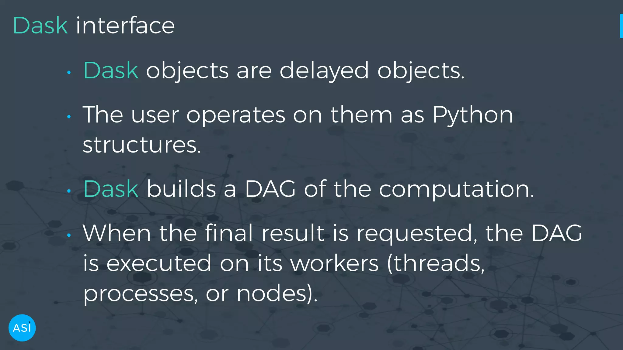
Dask interface • Dask objects are delayed objects. • The user operates on them as Python structures. • Dask builds a DAG of the computation. • When the final result is requested, the DAG is executed on its workers (threads, processes, or nodes).
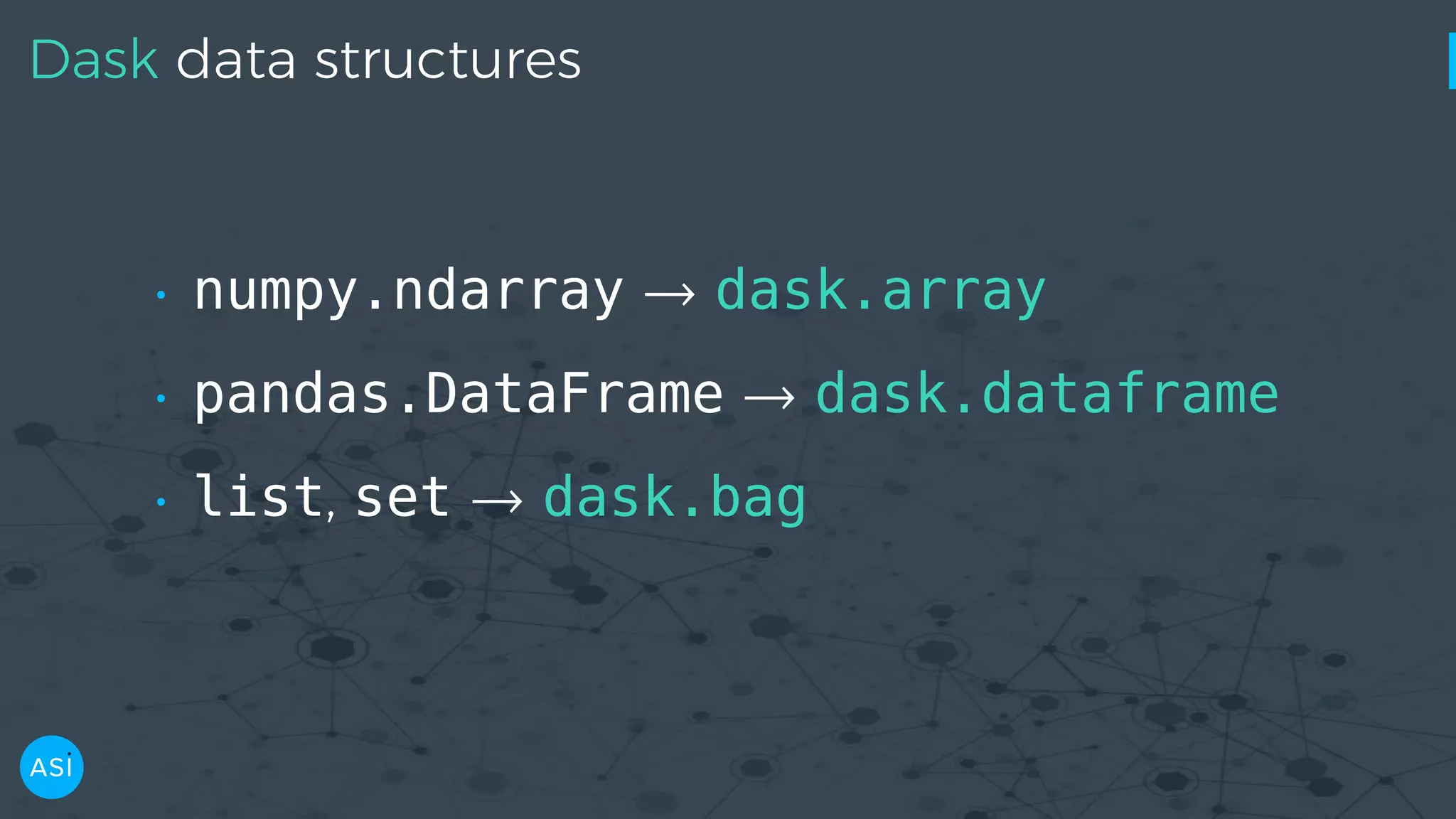
Dask data structures • numpy.ndarray → dask.array • pandas.DataFrame → dask.dataframe • list, set → dask.bag
dask.delayed — Build you own DAG files = ['myfile.a.data', 'myfile.b.data', 'myfile.c.data'] loaded = [load(i) for i in files] cleaned = [clean(i) for i in loaded] analyzed = analyze(cleaned) store(analyzed)
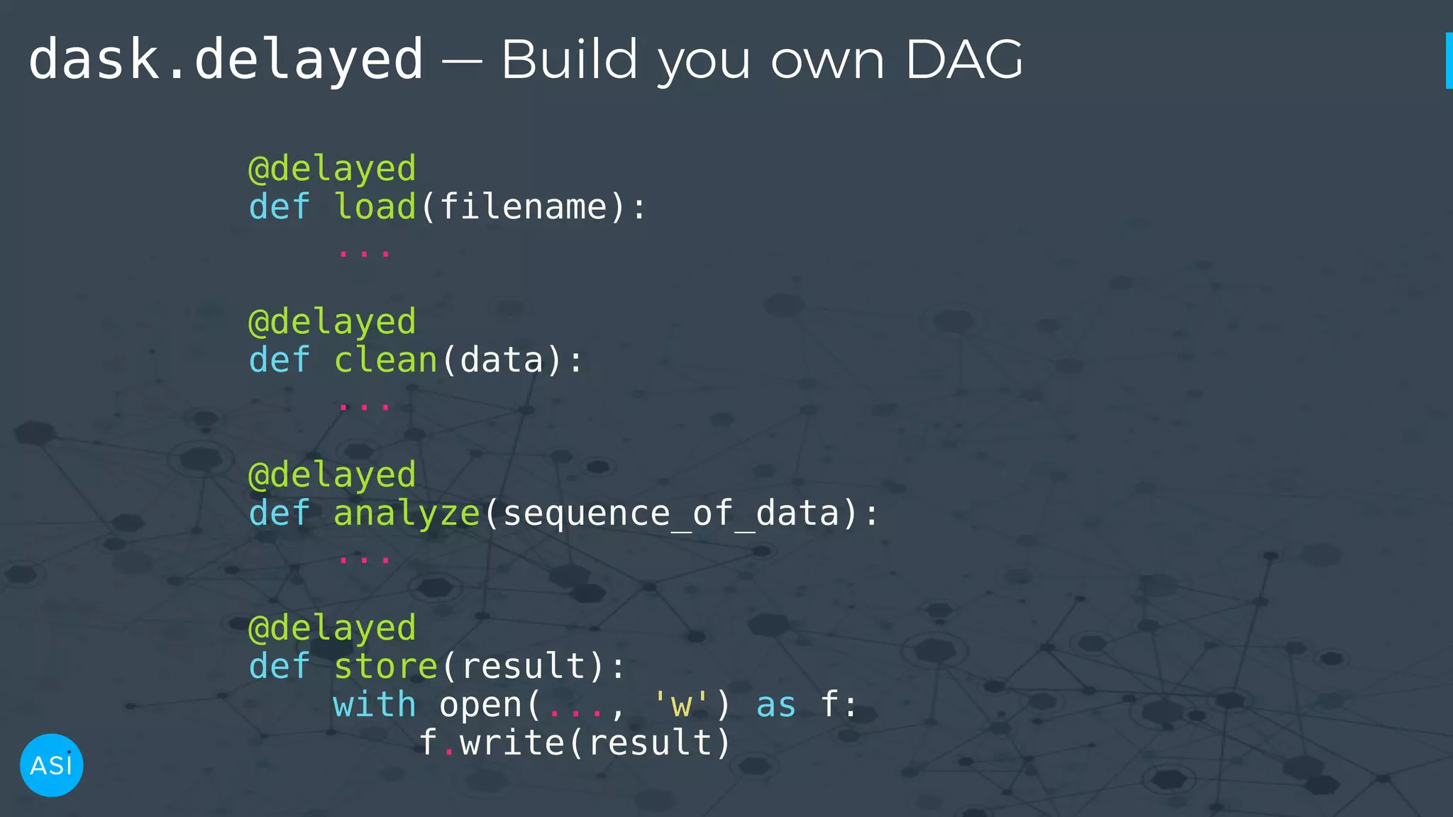
dask.delayed — Build you own DAG @delayed def load(filename): ... @delayed def clean(data): ... @delayed def analyze(sequence_of_data): ... @delayed def store(result): with open(..., 'w') as f: f.write(result)
dask.delayed — Build you own DAG files = ['myfile.a.data', 'myfile.b.data', 'myfile.c.data'] loaded = [load(i) for i in files] cleaned = [clean(i) for i in loaded] analyzed = analyze(cleaned) stored = store(analyzed) clean-2 analyze cleanload-2 analyze store clean-3 clean-1 load storecleanload-1 cleanload-3load load stored.compute()
Dask DAG execution In memory Released from memory
Comparison with PySpark • Native Python — better interaction with Python libraries • Easy deployment • Focused on arbitrary graphs • Optimized for • low latency • low memory usage
How do we use Dask in Lens?
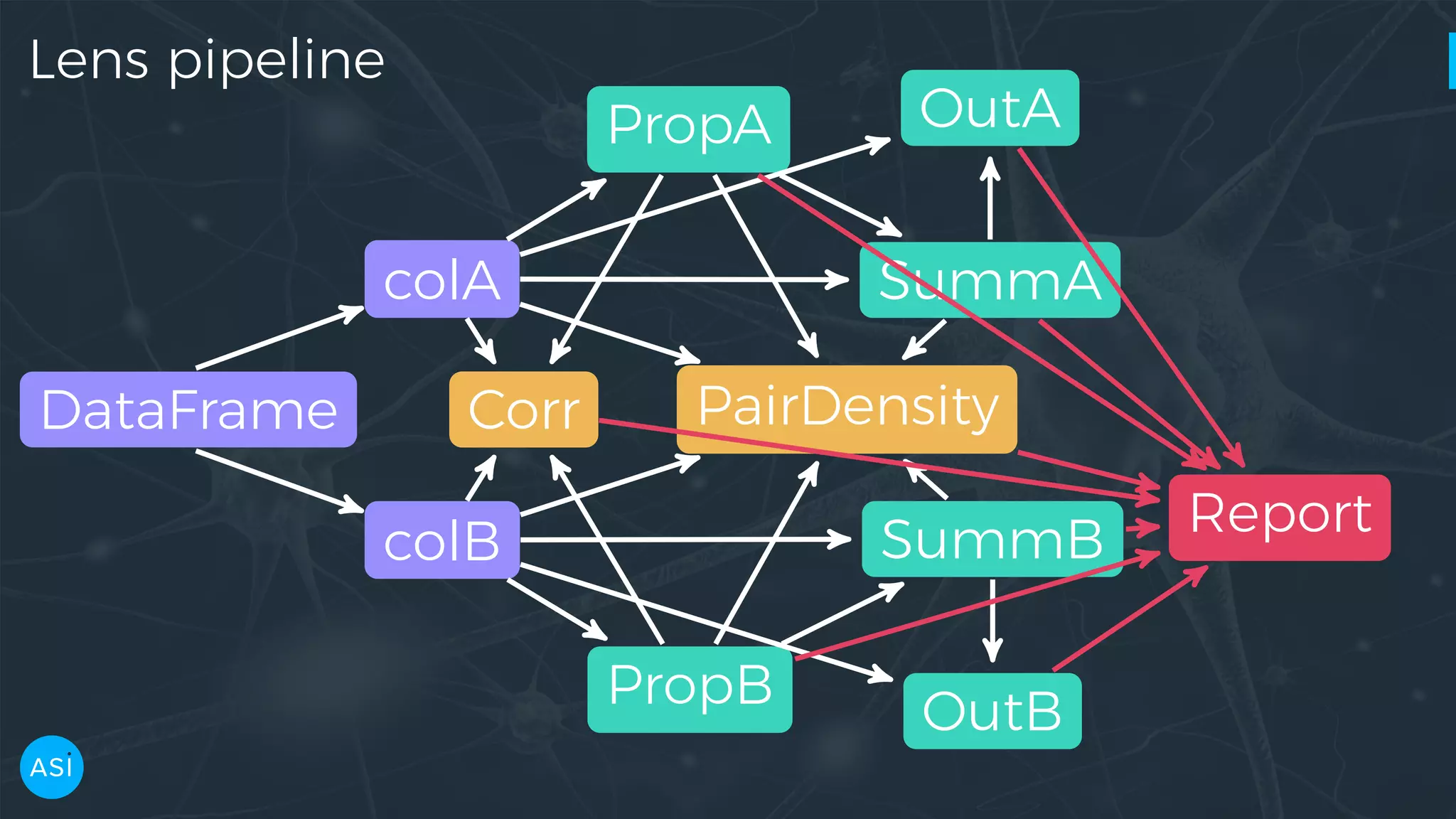
Lens pipeline DataFrame colA colB PropA PropB SummA SummB OutA OutB Corr PairDensity Report
Building the graph with dask.delayed # Create a series for each column in the DataFrame. columns = df.columns df = delayed(df) cols = {k: delayed(df.get)(k) for k in columns} # Create the delayed reports using Dask. cprops = {k: delayed(metrics.column_properties)(cols[k]) for k in columns} csumms = {k: delayed(metrics.column_summary)(cols[k], cprops[k]) for k in columns} corr = delayed(metrics.correlation)(df, cprops)
Building the graph with dask.delayed pdens_results = [] if pairdensities: for col1, col2 in itertools.combinations(columns, 2): pdens_df = delayed(pd.concat)([cols[col1], cols[col2]]) pdens_cp = {k: cprops[k] for k in [col1, col2]} pdens_cs = {k: csumms[k] for k in [col1, col2]} pdens_fr = {k: freqs[k] for k in [col1, col2]} pdens = delayed(metrics.pairdensity)( pdens_df, pdens_cp, pdens_cs, pdens_fr) pdens_results.append(pdens) # Join the delayed per-metric reports into a dictionary. report = delayed(dict)(column_properties=cprops, column_summary=csumms, pair_density=pdens_results, ...) return report
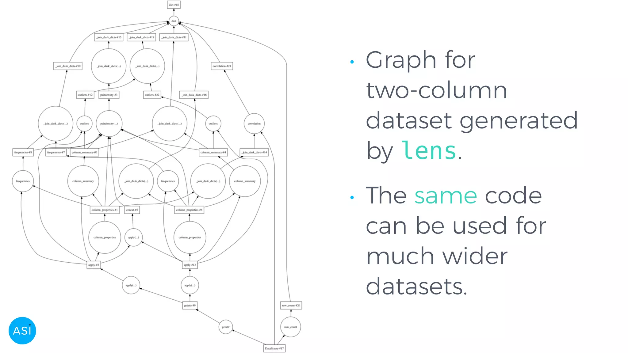
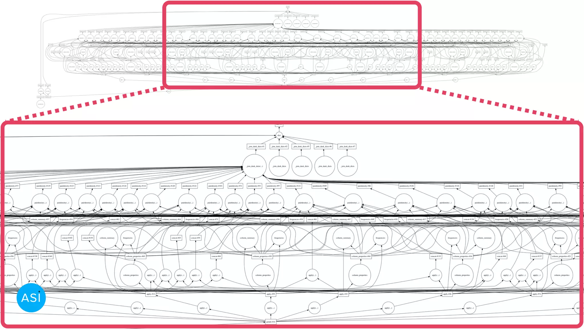
• Graph for two-column dataset generated by lens. • The same code can be used for much wider datasets.
Integration with infrastructure
SherlockML integration • Every dataset entering the platform is analysed by Lens. • We can use the same Python library! • The web frontend is used to interact with datasets.
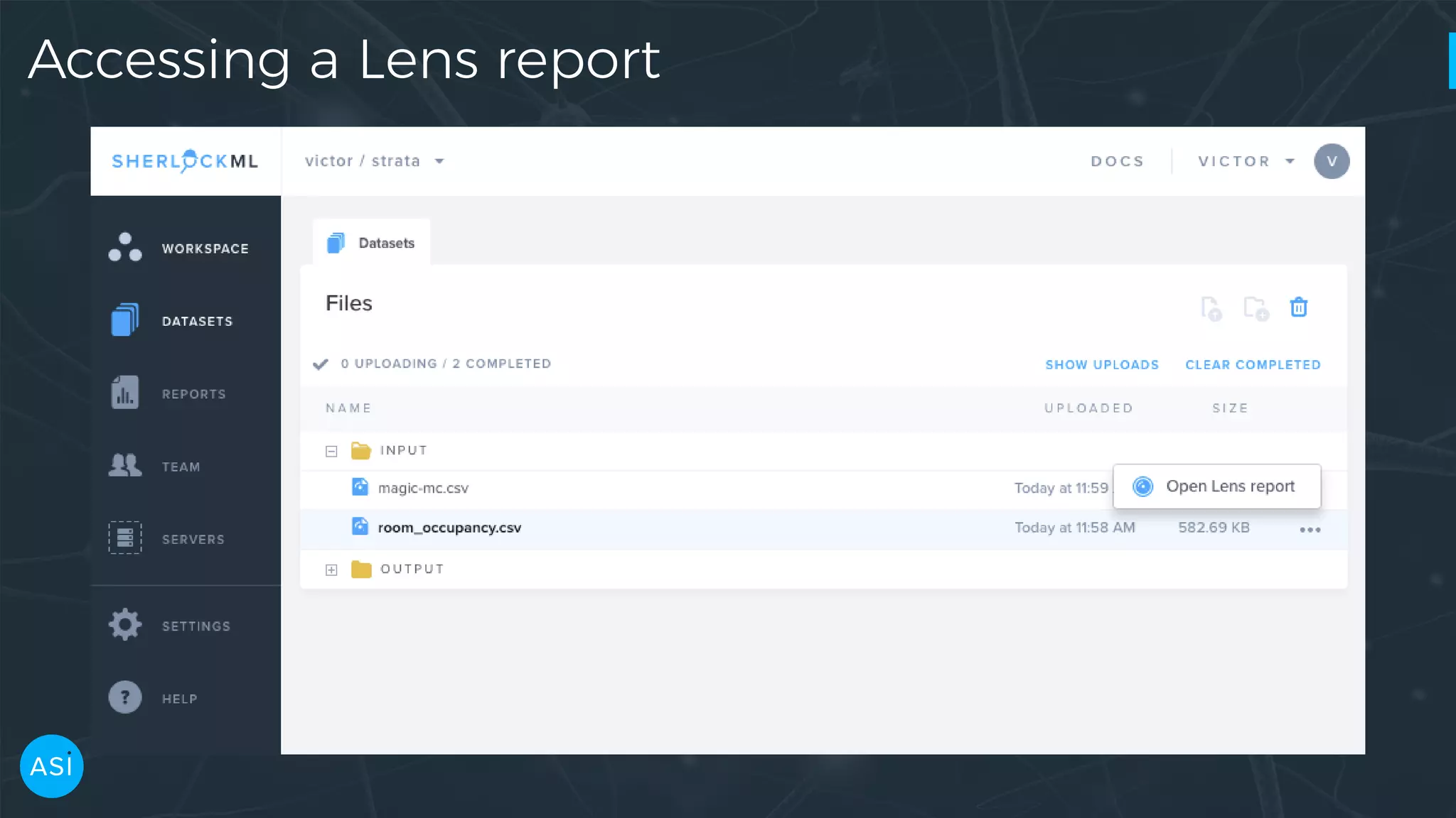
Accessing a Lens report
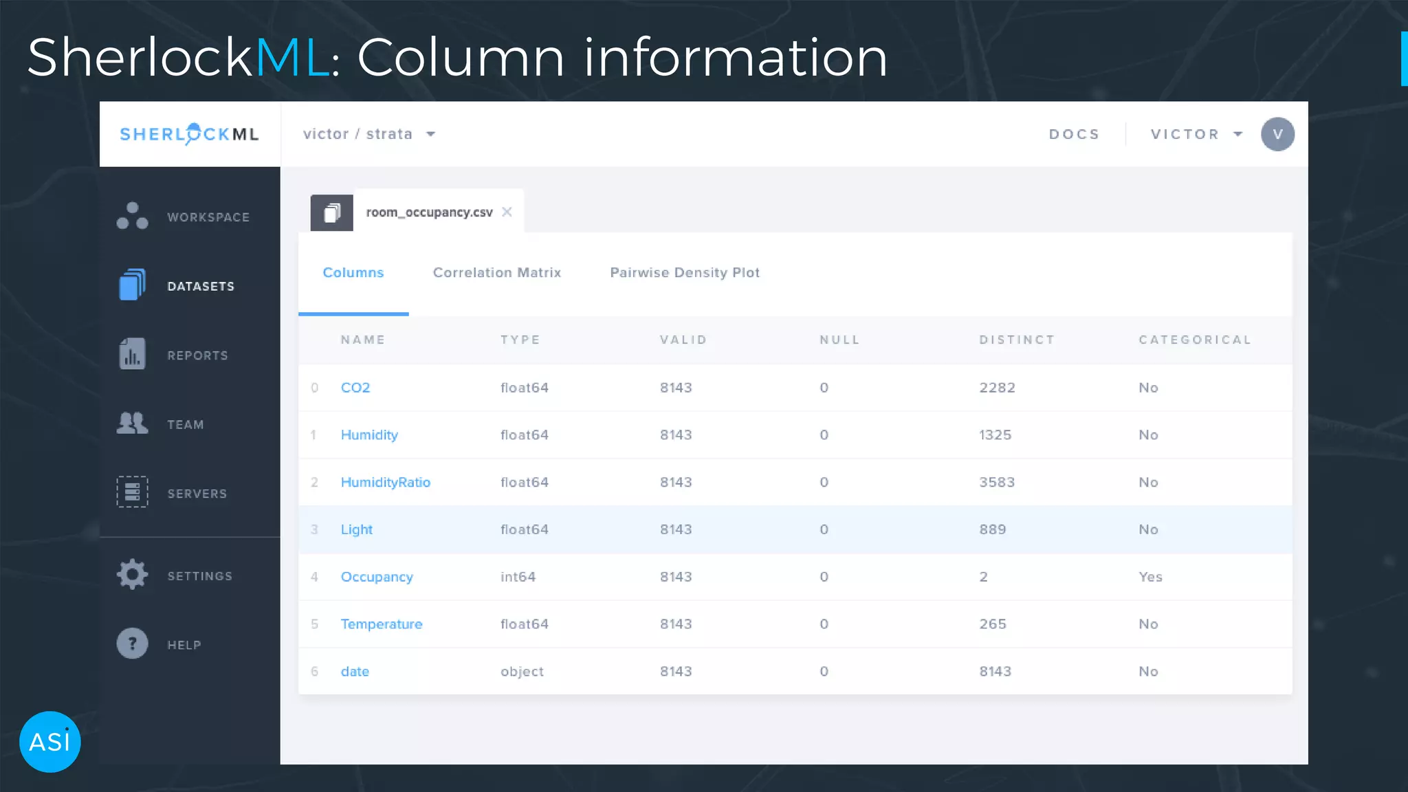
SherlockML: Column information
SherlockML: Column distribution
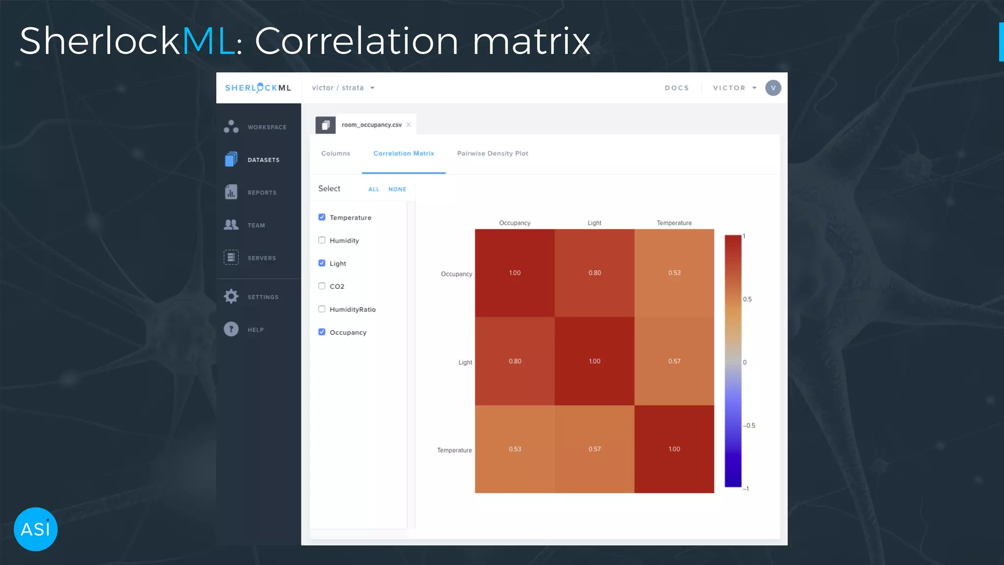
SherlockML: Correlation matrix
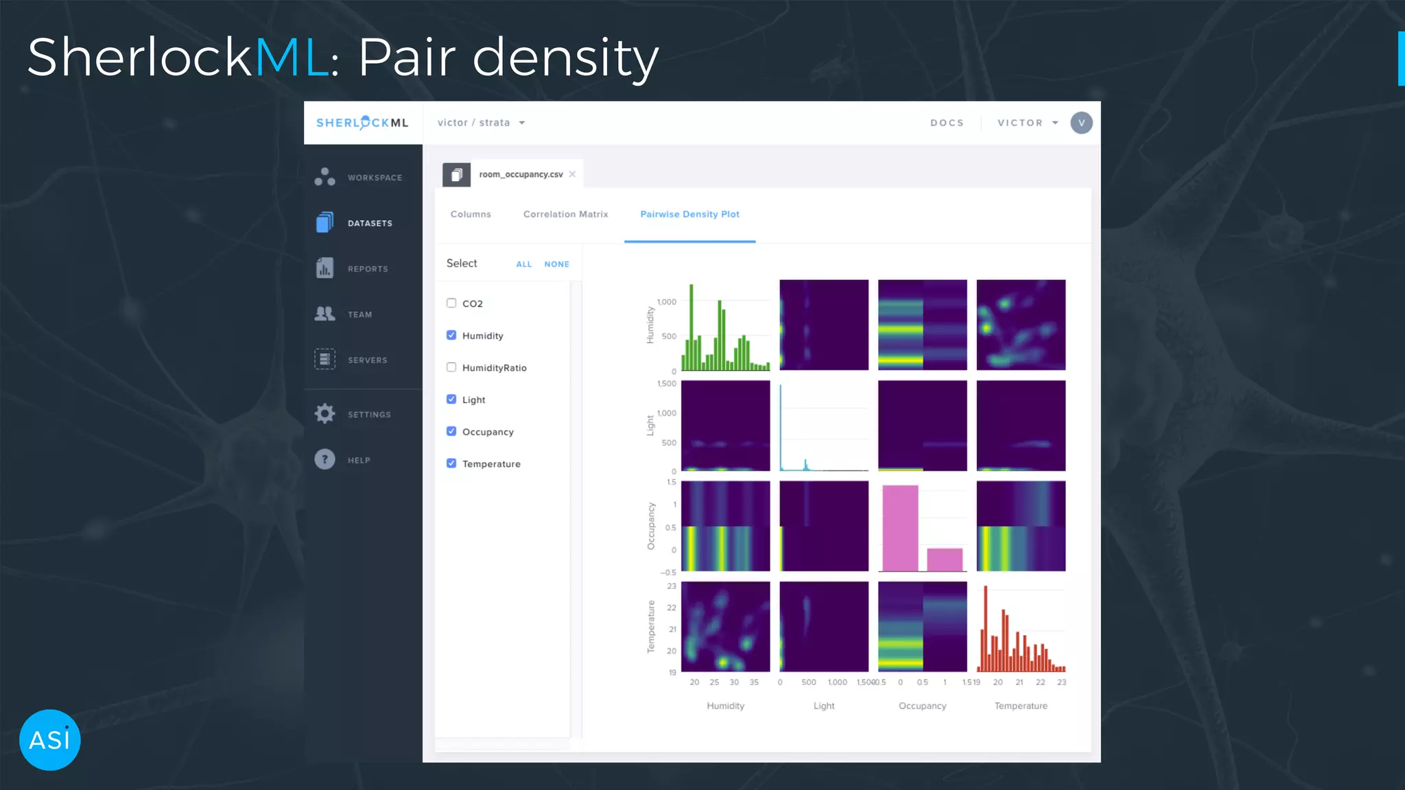
SherlockML: Pair density
Lens • Keeps interactive exploration snappy by splitting computation and exploration. • Upfront computation leverages dask to scale. • Easy exploration no matter the data size! • Keep your data scientists happy and productive.
Lens • Lens will be open source. • You can use the library and service right now on SherlockML.
Copyright © ASI 2016 All rights reserved ✓ Secure Scalable Compute ✓ Rapid Exploration and Cleaning ✓ Easy Collaboration ✓ Clear Communication LONDON IRISH SecurePowerful Simple
https://sherlockml.com Invite code: Strata2017

Automated Data Exploration: Building efficient analysis pipelines with Dask

  • 1.
    Automated Data Exploration Buildingefficient analysis pipelines with Dask Víctor Zabalza victor.z@asidatascience.com @zblz @ASIDataScience
  • 2.
    About me • Dataengineer at ASI Data Science. • Former astrophysicist. • Main developer of naima, a Python package for radiative analysis of non-thermal astronomical sources. • matplotlib developer.
  • 3.
    ASI Data Science •Data science consultancy • Academia to Data Industry fellowship • SherlockML
  • 4.
  • 5.
    First steps ina Data Science project • Does the data fit in a single computer? • Data quality assessment • Data exploration • Data cleaning
  • 6.
  • 8.
    Can we automatethe drudge work?
  • 9.
    Developing a toolfor data exploration based on Dask
  • 10.
    Lens Library and servicefor automated data quality assessment and exploration
  • 11.
    Lens by example Roomoccupancy dataset • ML standard dataset • Goal: predict occupancy based on ambient measurements. • What can we learn about it with Lens?
  • 12.
    Python interface >>> importlens >>> df = pd.read_csv('room_occupancy.csv') >>> ls = lens.summarise(df) >>> type(ls) <class 'lens.summarise.Summary'> >>> ls.to_json('room_occupancy_lens.json') room_occupancy_lens.json now contains all information needed for exploration!
  • 13.
    Python interface —Columns >>> ls = lens.Summary.from_json('room_occupancy_lens.json') >>> ls.columns ['date', 'Temperature', 'Humidity', 'Light', 'CO2', 'HumidityRatio', 'Occupancy']
  • 14.
    Python interface —Categorical summary >>> ls.summary('Occupancy') {'name': 'Occupancy', 'desc': 'categorical', 'dtype': 'int64', 'nulls': 0, 'notnulls': 8143, 'unique': 2} >>> ls.details('Occupancy') {'desc': 'categorical', 'frequencies': {0: 6414, 1: 1729}, 'name': 'Occupancy'}
  • 15.
    Python interface —Numeric summary >>> ls.details('Temperature') {'name': 'Temperature', 'desc': 'numeric', 'iqr': 1.69, 'min': 19.0, 'max': 23.18, 'mean': 20.619, 'median': 20.39, 'std': 1.0169, 'sum': 167901.1980}
  • 16.
    Python interface —KDE, PDF >>> x, y = ls.kde('Temperature') >>> x[np.argmax(y)] 19.417999999999999 >>> temperature_pdf = ls.pdf('Temperature') >>> temperature_pdf([19, 20, 21, 22]) array([ 0.01754398, 0.76491742, 0.58947765, 0.28421244])
  • 17.
    The lens.Summary isa good building block, but clunky for exploration. Can we do better?
  • 18.
  • 19.
  • 20.
  • 21.
  • 22.
  • 23.
  • 24.
  • 25.
  • 26.
  • 27.
  • 28.
    Requirements • Versatile • Reproducible •Portable • Scalable • Reusable
  • 29.
    Our solution: Analysis •A Python library computes dataset metrics: • Column-wise statistics • Pairwise densities • ... • Computation cost is paid up front. • The result is serialized to JSON.
  • 30.
    Our Solution: Interactiveexploration • Using only the report, the user can explore the dataset through either: • Jupyter widgets • Web UI
  • 31.
  • 32.
    Why Python? Portability APython library easily runs in: • Jupyter notebooks for interactive analysis. • One-off scripts. • Scheduled or on-demand jobs in cluster.
  • 33.
    Why Python? Reusability •Allows us to use the Python data ecosystem. • Becomes a building block in the Data Science process.
  • 34.
    Why Python? Scalability •Python is great for single-core, in-memory, numerical computations through numpy, scipy, pandas. • But the GIL limits its ability to parallelise workloads. Can Python scale?
  • 35.
    Out-of-core options inPython Difficult Flexible Easy Restrictive Threads, Processes, MPI, ZeroMQ Concurrent.futures, joblib Luigi PySpark Hadoop, SQL Dask
  • 36.
  • 37.
    Dask interface • Daskobjects are delayed objects. • The user operates on them as Python structures. • Dask builds a DAG of the computation. • When the final result is requested, the DAG is executed on its workers (threads, processes, or nodes).
  • 38.
    Dask data structures •numpy.ndarray → dask.array • pandas.DataFrame → dask.dataframe • list, set → dask.bag
  • 39.
    dask.delayed — Buildyou own DAG files = ['myfile.a.data', 'myfile.b.data', 'myfile.c.data'] loaded = [load(i) for i in files] cleaned = [clean(i) for i in loaded] analyzed = analyze(cleaned) store(analyzed)
  • 40.
    dask.delayed — Buildyou own DAG @delayed def load(filename): ... @delayed def clean(data): ... @delayed def analyze(sequence_of_data): ... @delayed def store(result): with open(..., 'w') as f: f.write(result)
  • 41.
    dask.delayed — Buildyou own DAG files = ['myfile.a.data', 'myfile.b.data', 'myfile.c.data'] loaded = [load(i) for i in files] cleaned = [clean(i) for i in loaded] analyzed = analyze(cleaned) stored = store(analyzed) clean-2 analyze cleanload-2 analyze store clean-3 clean-1 load storecleanload-1 cleanload-3load load stored.compute()
  • 42.
    Dask DAG execution Inmemory Released from memory
  • 43.
    Comparison with PySpark •Native Python — better interaction with Python libraries • Easy deployment • Focused on arbitrary graphs • Optimized for • low latency • low memory usage
  • 44.
    How do weuse Dask in Lens?
  • 45.
  • 46.
    Building the graphwith dask.delayed # Create a series for each column in the DataFrame. columns = df.columns df = delayed(df) cols = {k: delayed(df.get)(k) for k in columns} # Create the delayed reports using Dask. cprops = {k: delayed(metrics.column_properties)(cols[k]) for k in columns} csumms = {k: delayed(metrics.column_summary)(cols[k], cprops[k]) for k in columns} corr = delayed(metrics.correlation)(df, cprops)
  • 47.
    Building the graphwith dask.delayed pdens_results = [] if pairdensities: for col1, col2 in itertools.combinations(columns, 2): pdens_df = delayed(pd.concat)([cols[col1], cols[col2]]) pdens_cp = {k: cprops[k] for k in [col1, col2]} pdens_cs = {k: csumms[k] for k in [col1, col2]} pdens_fr = {k: freqs[k] for k in [col1, col2]} pdens = delayed(metrics.pairdensity)( pdens_df, pdens_cp, pdens_cs, pdens_fr) pdens_results.append(pdens) # Join the delayed per-metric reports into a dictionary. report = delayed(dict)(column_properties=cprops, column_summary=csumms, pair_density=pdens_results, ...) return report
  • 48.
    • Graph for two-column datasetgenerated by lens. • The same code can be used for much wider datasets.
  • 50.
  • 51.
    SherlockML integration • Everydataset entering the platform is analysed by Lens. • We can use the same Python library! • The web frontend is used to interact with datasets.
  • 52.
  • 53.
  • 54.
  • 55.
  • 56.
  • 57.
    Lens • Keeps interactiveexploration snappy by splitting computation and exploration. • Upfront computation leverages dask to scale. • Easy exploration no matter the data size! • Keep your data scientists happy and productive.
  • 58.
    Lens • Lens willbe open source. • You can use the library and service right now on SherlockML.
  • 59.
    Copyright © ASI2016 All rights reserved ✓ Secure Scalable Compute ✓ Rapid Exploration and Cleaning ✓ Easy Collaboration ✓ Clear Communication LONDON IRISH SecurePowerful Simple
  • 60.