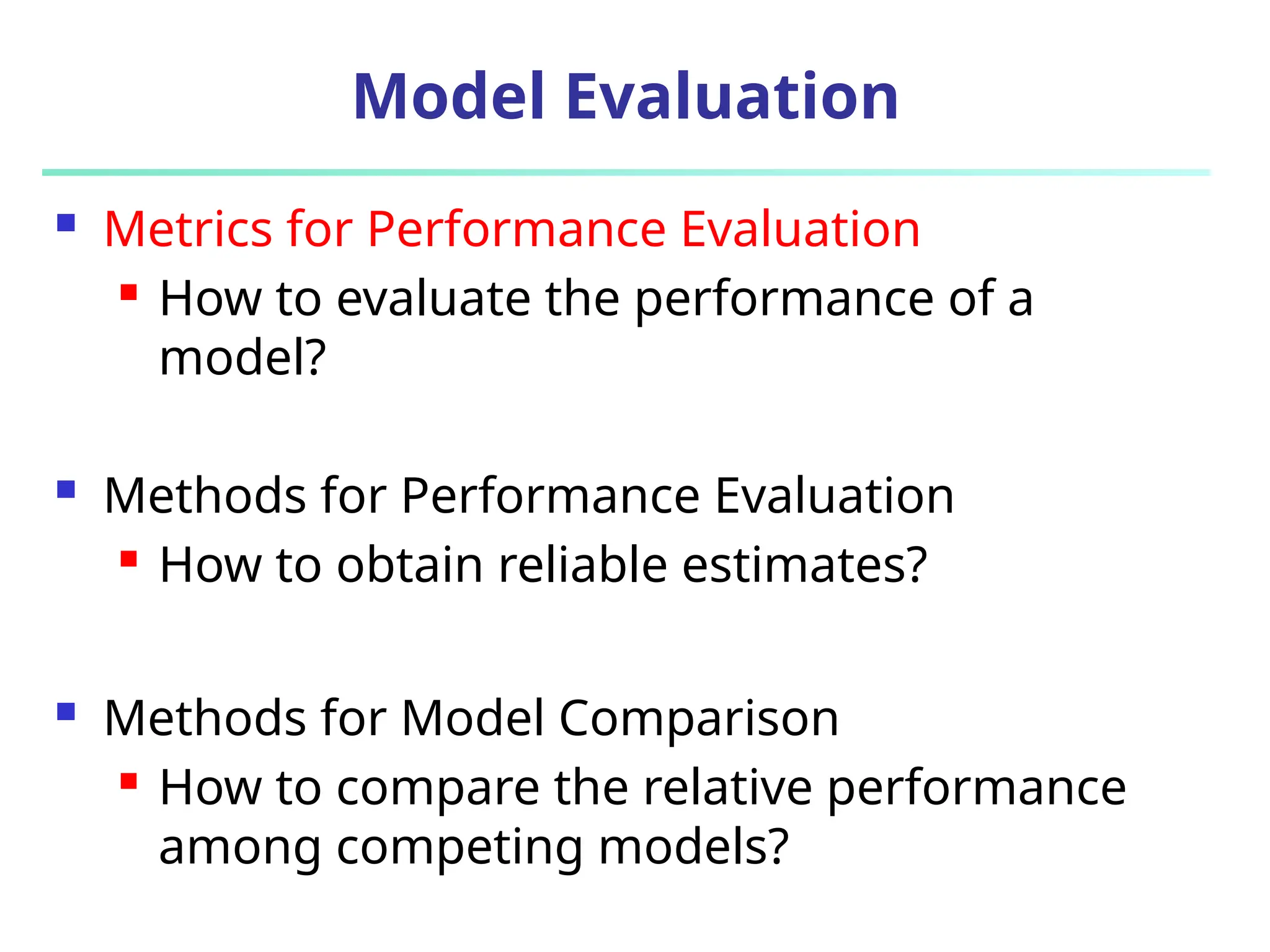
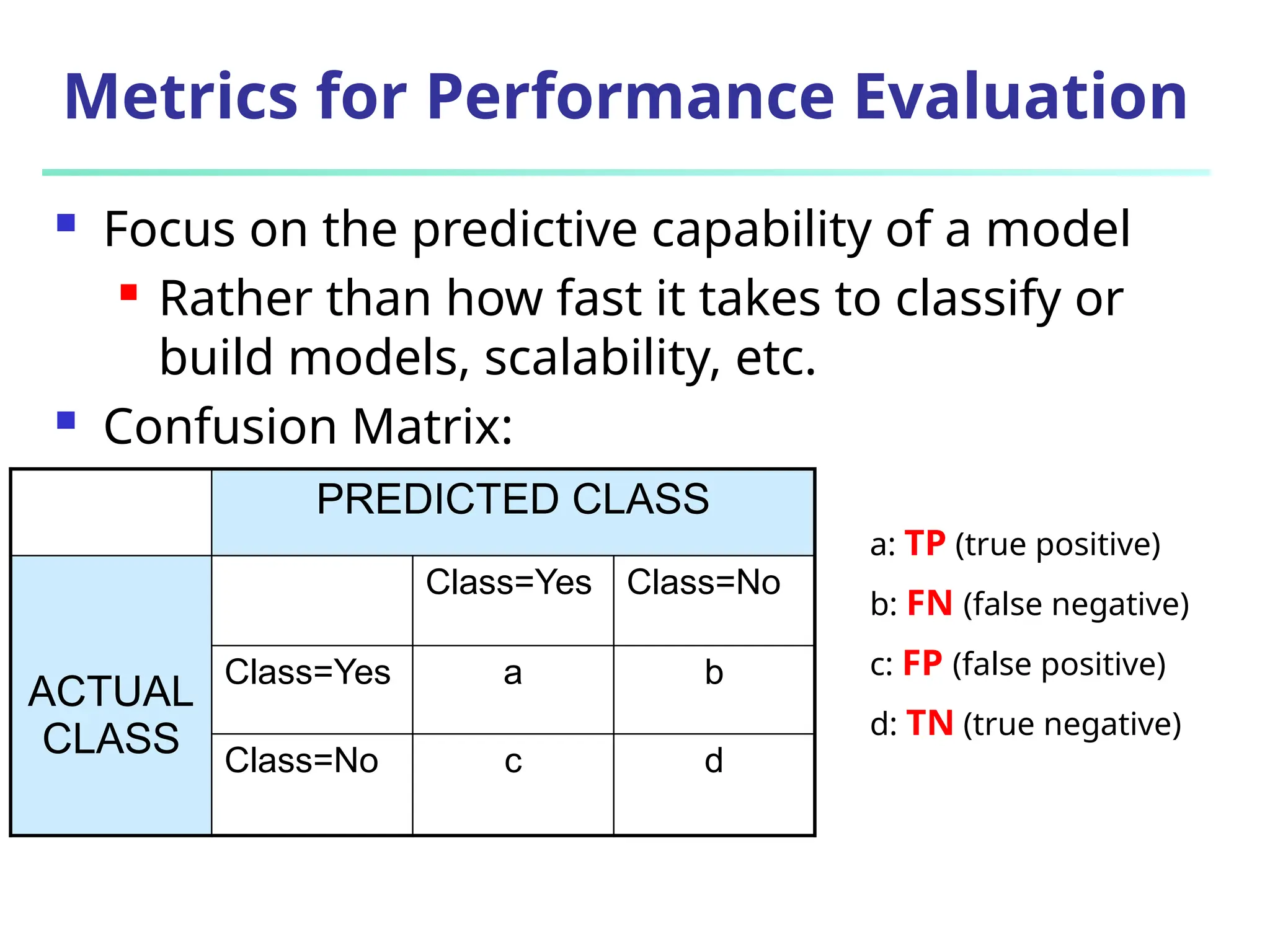
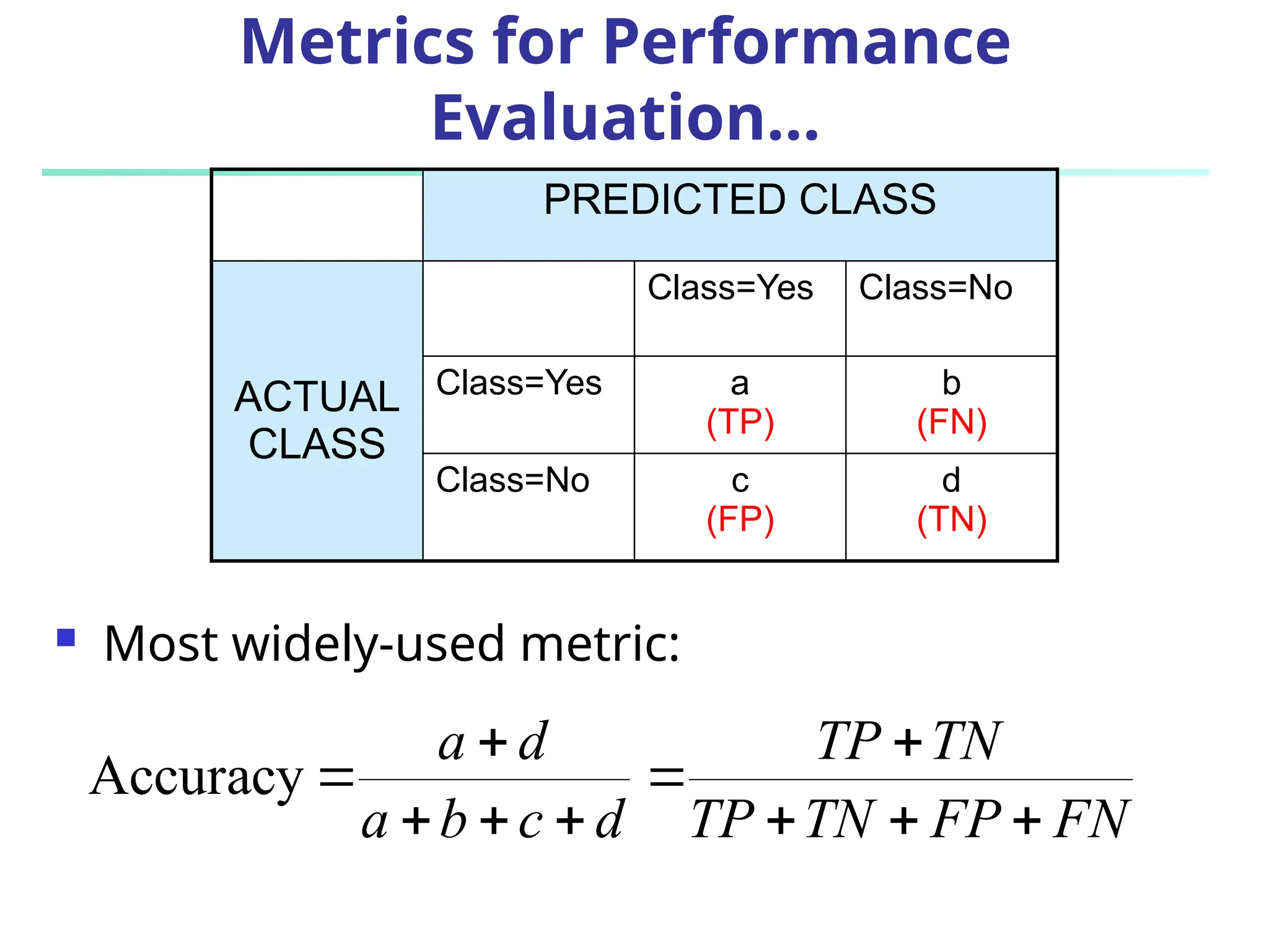
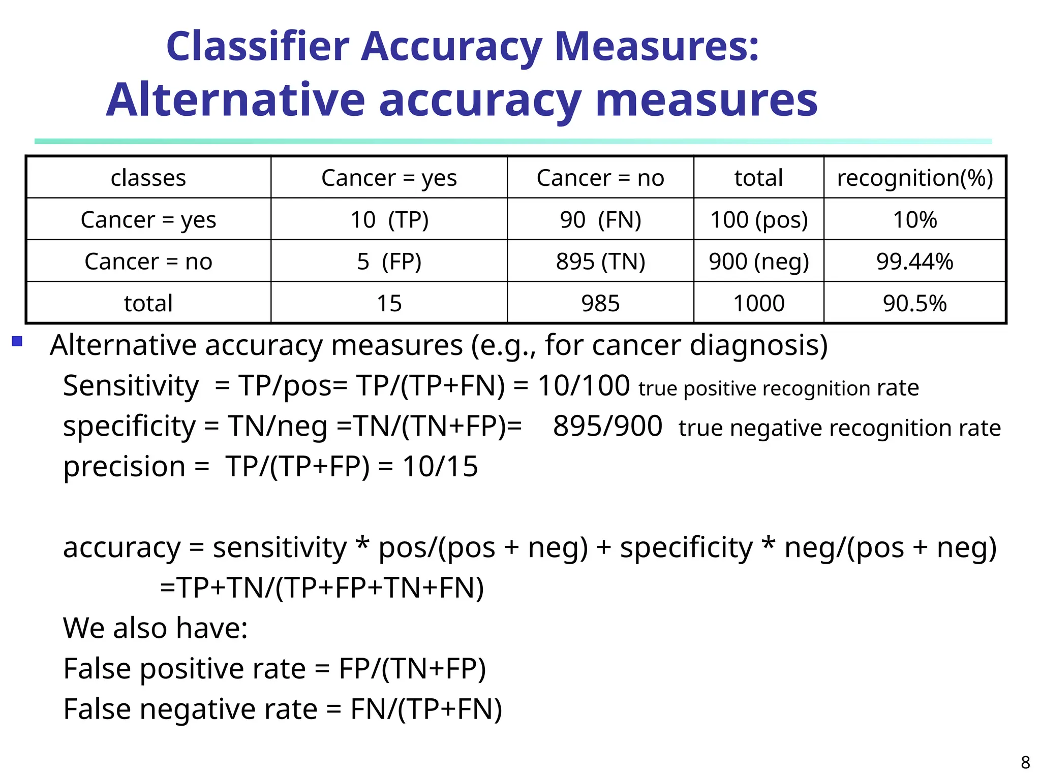
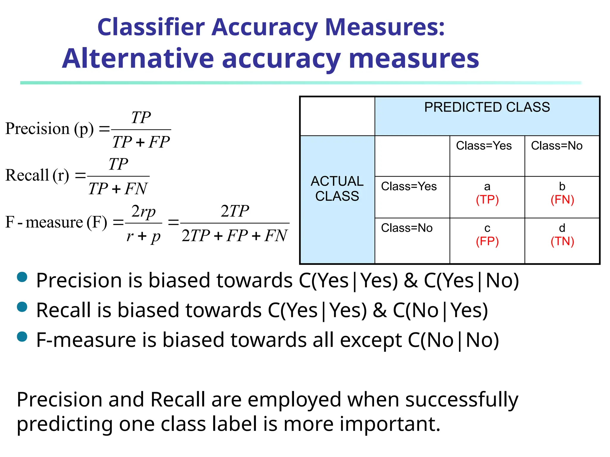
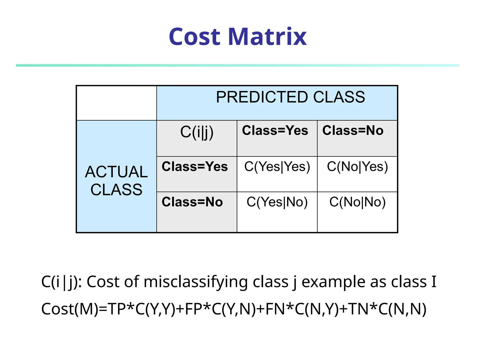
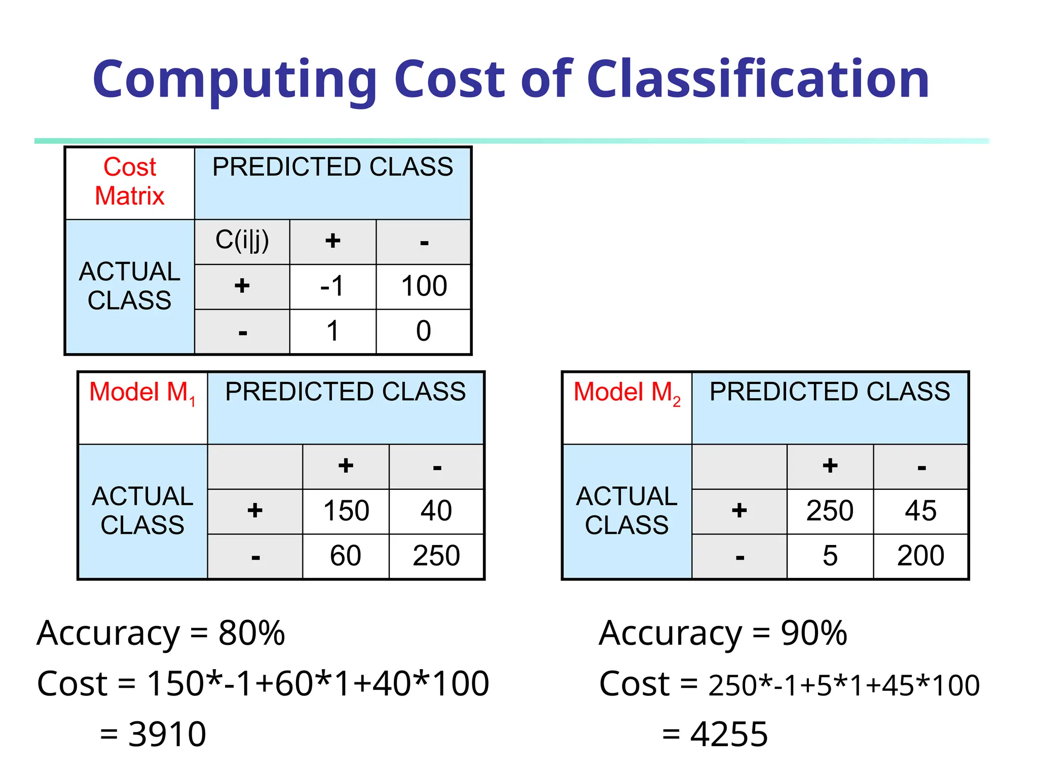
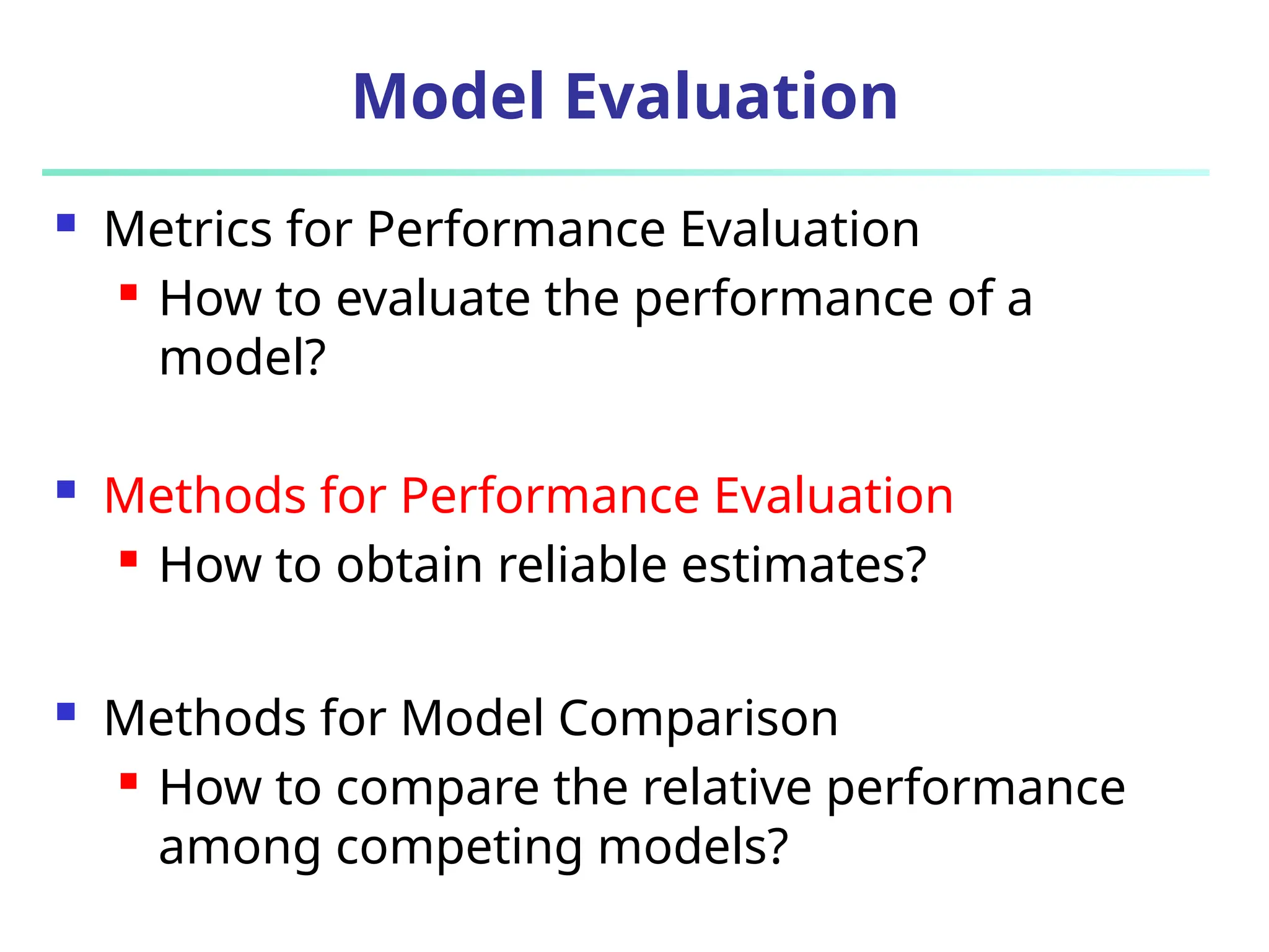
Classification in data mining from lectures

Introduction to Data Mining Classification 1 These slides are based on slides by 1) Jiawei Han and Micheline Kamber 2) Tan, Stienback, and Kumar 3) Mohammed Zaki

Model Evaluation  Metrics for Performance Evaluation  How to evaluate the performance of a model?  Methods for Performance Evaluation  How to obtain reliable estimates?  Methods for Model Comparison  How to compare the relative performance among competing models?

Metrics for Performance Evaluation  Focus on the predictive capability of a model  Rather than how fast it takes to classify or build models, scalability, etc.  Confusion Matrix: PREDICTED CLASS ACTUAL CLASS Class=Yes Class=No Class=Yes a b Class=No c d a: TP (true positive) b: FN (false negative) c: FP (false positive) d: TN (true negative)

Metrics for Performance Evaluation…  Most widely-used metric: PREDICTED CLASS ACTUAL CLASS Class=Yes Class=No Class=Yes a (TP) b (FN) Class=No c (FP) d (TN) FN FP TN TP TN TP d c b a d a           Accuracy

Limitation of Accuracy  Consider a 2-class problem  Number of Class 0 examples = 9990  Number of Class 1 examples = 10  If model predicts everything to be class 0,

Limitation of Accuracy  Consider a 2-class problem  Number of Class 0 examples = 9990  Number of Class 1 examples = 10  If model predicts everything to be class 0, accuracy is 9990/10000 = 99.9 %  Accuracy is misleading because model does not detect any class 1 example

7 Classifier Accuracy Measures: Alternative accuracy measures  A high accuracy rate (90.5%) may not be acceptable!! classes Cancer = yes Cancer = no total recognition(%) Cancer = yes 10 (TP) 90 (FN) 100 (pos) 10% Cancer = no 5 (FP) 895 (TN) 900 (neg) 99.44% total 15 985 1000 90.5%

8 Classifier Accuracy Measures: Alternative accuracy measures  Alternative accuracy measures (e.g., for cancer diagnosis) Sensitivity = TP/pos= TP/(TP+FN) = 10/100 true positive recognition rate specificity = TN/neg =TN/(TN+FP)= 895/900 true negative recognition rate precision = TP/(TP+FP) = 10/15 accuracy = sensitivity * pos/(pos + neg) + specificity * neg/(pos + neg) =TP+TN/(TP+FP+TN+FN) We also have: False positive rate = FP/(TN+FP) False negative rate = FN/(TP+FN) classes Cancer = yes Cancer = no total recognition(%) Cancer = yes 10 (TP) 90 (FN) 100 (pos) 10% Cancer = no 5 (FP) 895 (TN) 900 (neg) 99.44% total 15 985 1000 90.5%

FN FP TP TP p r rp FN TP TP FP TP TP          2 2 2 (F) measure - F (r) Recall (p) Precision  Precision is biased towards C(Yes|Yes) & C(Yes|No)  Recall is biased towards C(Yes|Yes) & C(No|Yes)  F-measure is biased towards all except C(No|No) Precision and Recall are employed when successfully predicting one class label is more important. Classifier Accuracy Measures: Alternative accuracy measures PREDICTED CLASS ACTUAL CLASS Class=Yes Class=No Class=Yes a (TP) b (FN) Class=No c (FP) d (TN)

Computing Cost of Classification Cost Matrix PREDICTED CLASS ACTUAL CLASS C(i|j) + - + -1 100 - 1 0 Model M1 PREDICTED CLASS ACTUAL CLASS + - + 150 40 - 60 250 Model M2 PREDICTED CLASS ACTUAL CLASS + - + 250 45 - 5 200 Accuracy = 80% Cost = 150*-1+60*1+40*100 = 3910 Accuracy = 90% Cost = 250*-1+5*1+45*100 = 4255

Methods for Performance Evaluation  How to obtain a reliable estimate of performance?  Performance of a model may depend on other factors besides the learning algorithm:  Class distribution  Cost of misclassification  Size of training and test sets

14 Performance Evaluating  Holdout method  Given data is randomly partitioned into two independent sets  Training set (e.g., 2/3) for model construction  Test set (e.g., 1/3) for accuracy estimation Limitations:  Less data available for train  The model is dependent on the composition of the train and test datasets.  Training and Testing no longer independent (more in one, less in the other).  Random sampling: a variation of holdout  Repeat holdout k times, accuracy = avg. of the accuracies obtained

15 Performance Evaluating  Cross-validation (k-fold, where k = 10 is most popular)  P partition the data into k mutually exclusive subsets, each approximately equal size  At i-th iteration, use Di as test set and others as training set  Leave-one-out: k folds where k = # of tuples, for small sized data For Unbalanced Data:  Stratified cross-validation: folds are stratified so that class dist. in each fold is approx. the same as that in the initial data

16 Performance Evaluating  Bootstrap  Works well with small data sets  Samples the given training tuples uniformly with replacement  i.e., each time a tuple is selected, it is equally likely to be selected again and re-added to the training set  Several boostrap methods, and a common one is .632 boostrap  Suppose we are given a data set of N tuples. Sample N times  training data tuples not in the trianing data  test data  About 63.2% of the original data will end up in the bootstrap, and the remaining 36.8% will form the test set (since (1 – 1/N)N e ≈ -1 = 0.368)  Repeat the sampling procedue k times, overall accuracy of the model:

Classification in data mining from lectures

More Related Content

Similar to Classification in data mining from lectures

Recently uploaded

Classification in data mining from lectures