DIGITAL IMAGE PROCESSING - Day 4 Image Transform

Digital Image Processing Day 4 : 25/6/2020 Agenda : Two Dimensional Mathematical Preliminaries 2D transforms 1) DFT- Discrete Fourier Transform 2) DCT - Discrete Cosine Transform

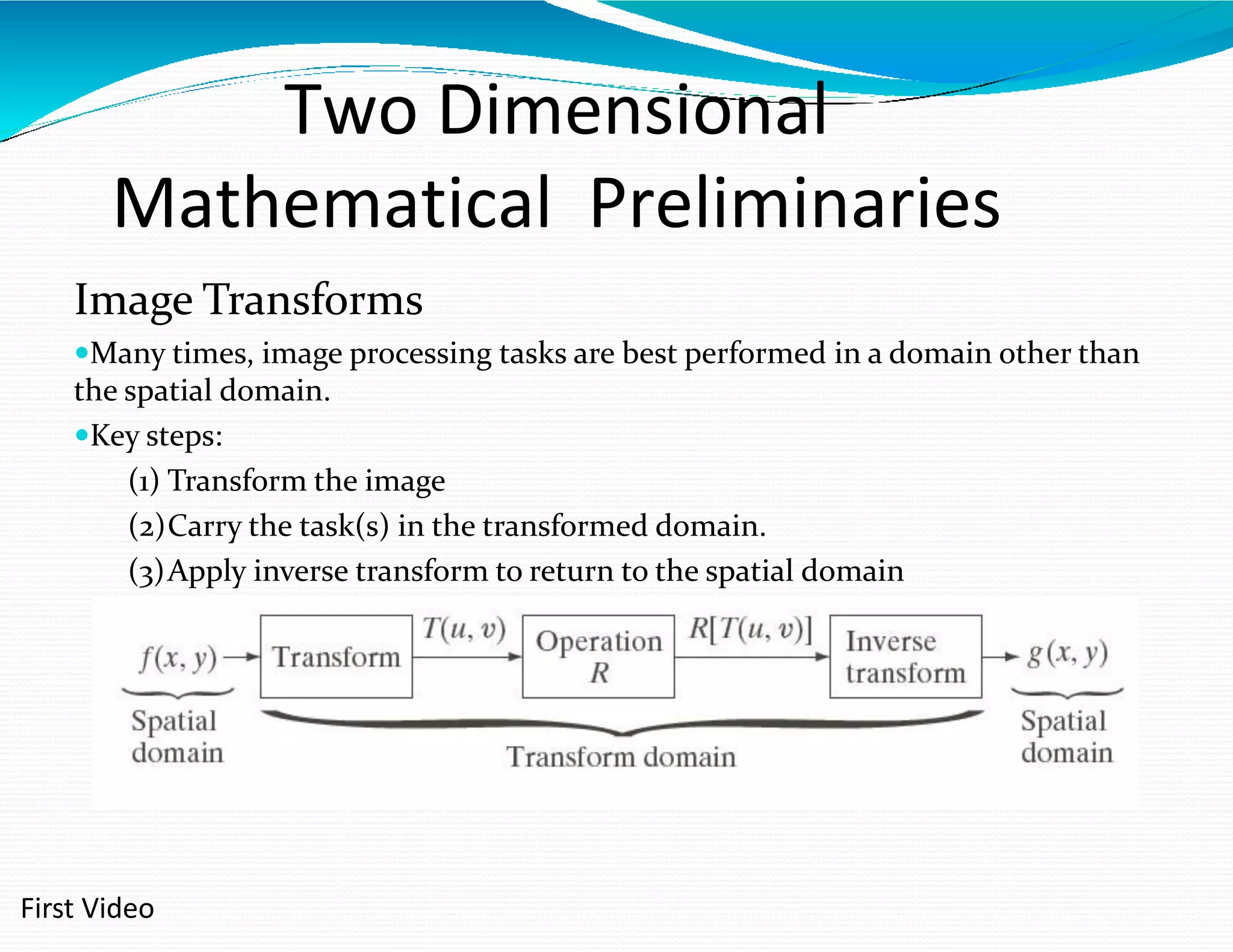
Two Dimensional Mathematical Preliminaries Image Transforms Many times, image processing tasks are best performed in a domain other than the spatial domain. Key steps: (1) Transform the image (2)Carry the task(s) in the transformed domain. (3)Apply inverse transform to return to the spatial domain First Video

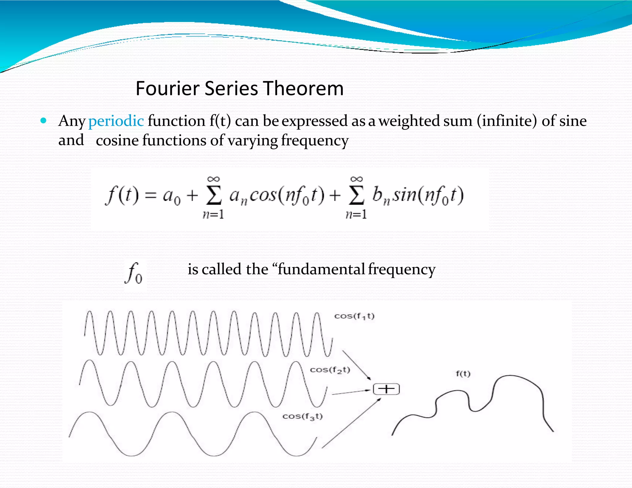
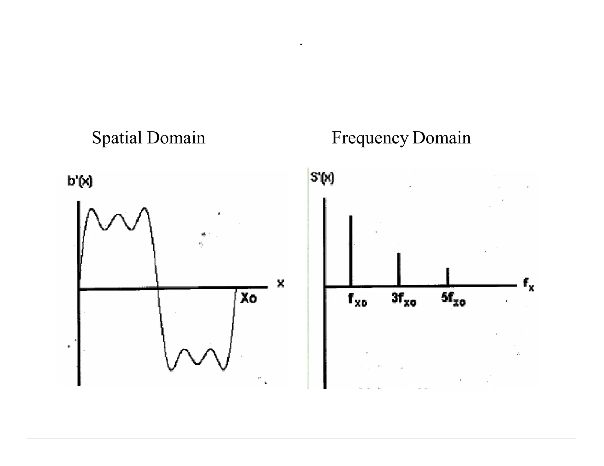
Fourier Series Theorem  Anyperiodic function f(t) can beexpressed as aweighted sum (infinite) of sine and cosine functions of varying frequency is called the “fundamentalfrequency

Discrete Fourier Transform (DFT)

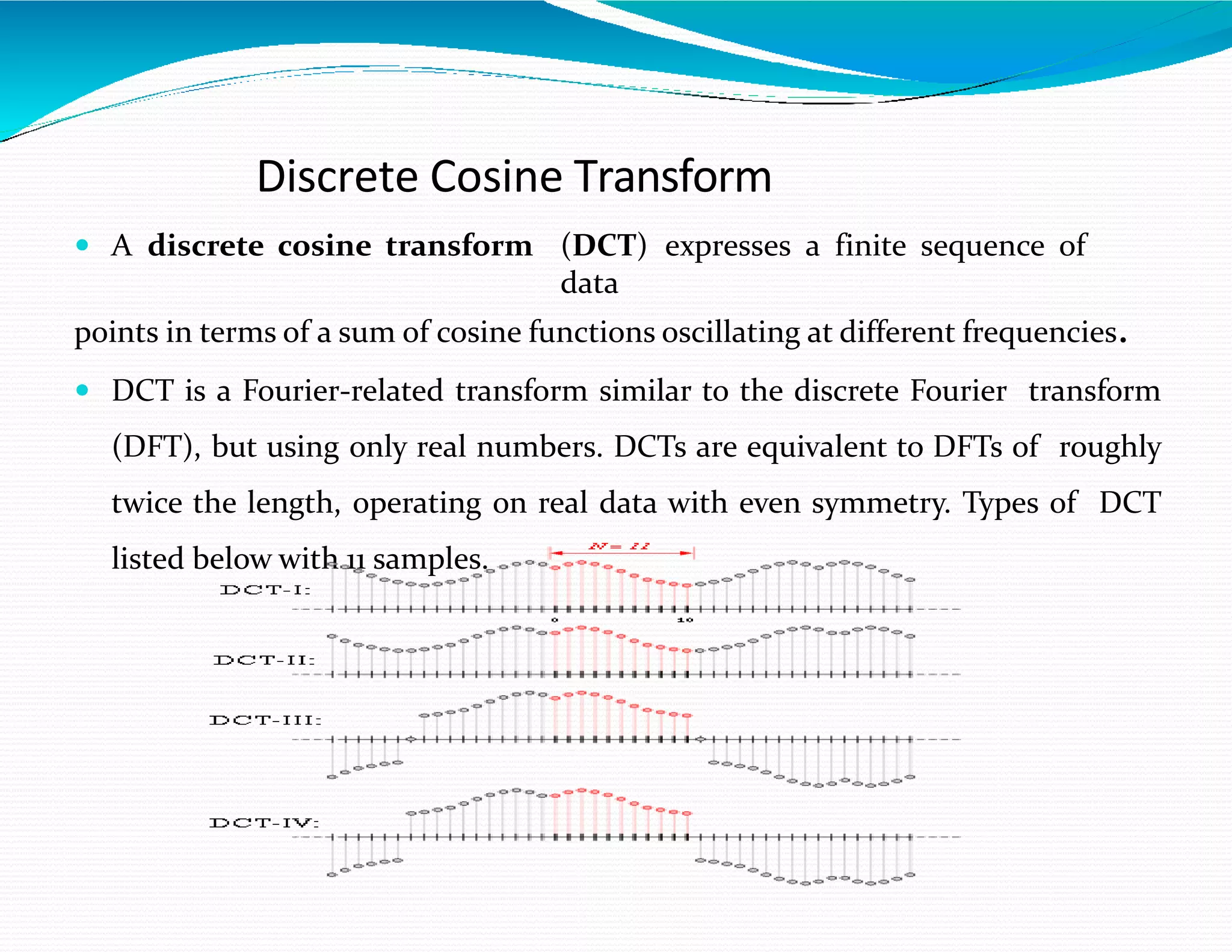
Discrete Cosine Transform  A discrete cosine transform (DCT) expresses a finite sequence of data points in terms of a sum of cosine functions oscillating at different frequencies.  DCT is a Fourier-related transform similar to the discrete Fourier transform (DFT), but using only real numbers. DCTs are equivalent to DFTs of roughly twice the length, operating on real data with even symmetry. Types of DCT listed below with 11 samples.

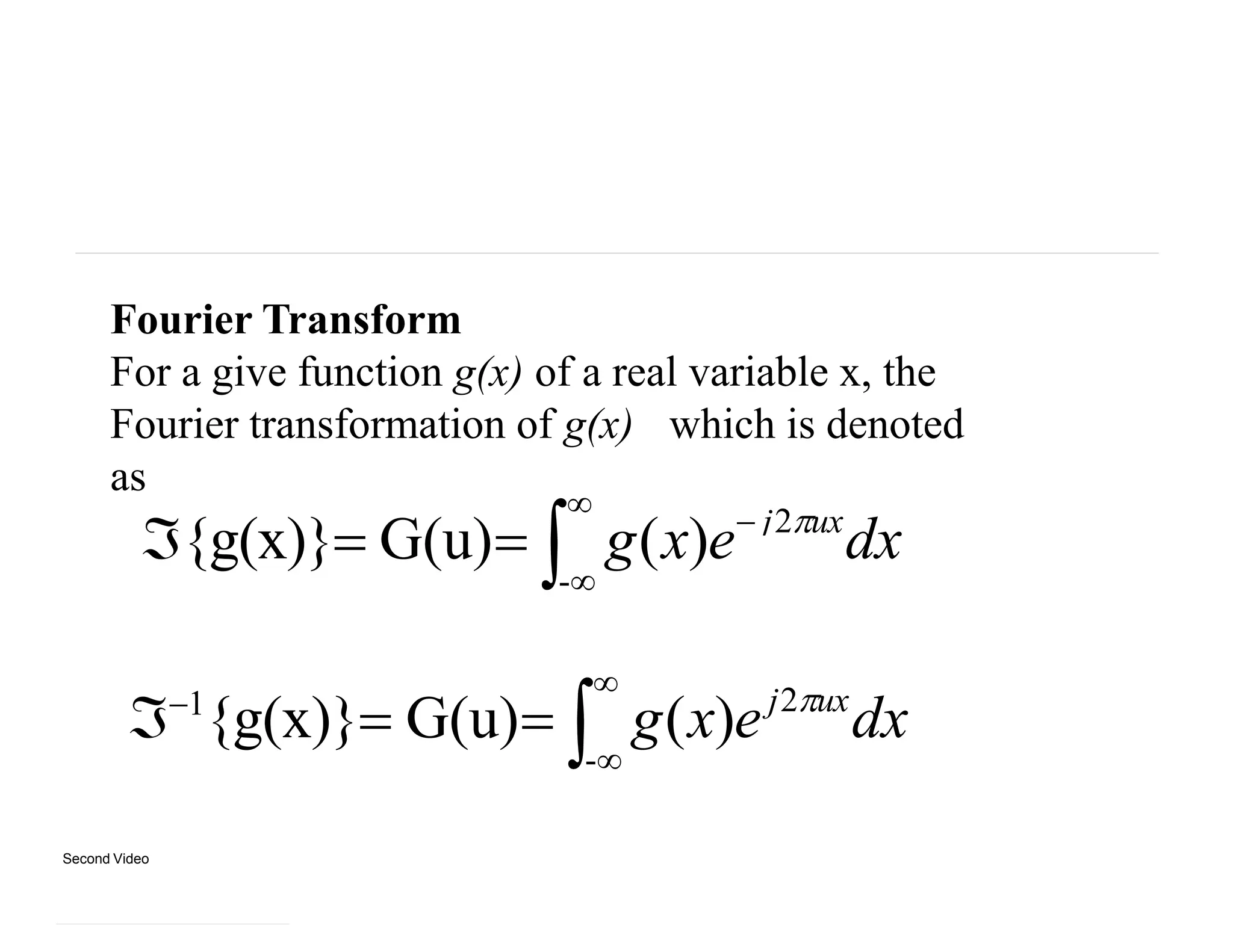
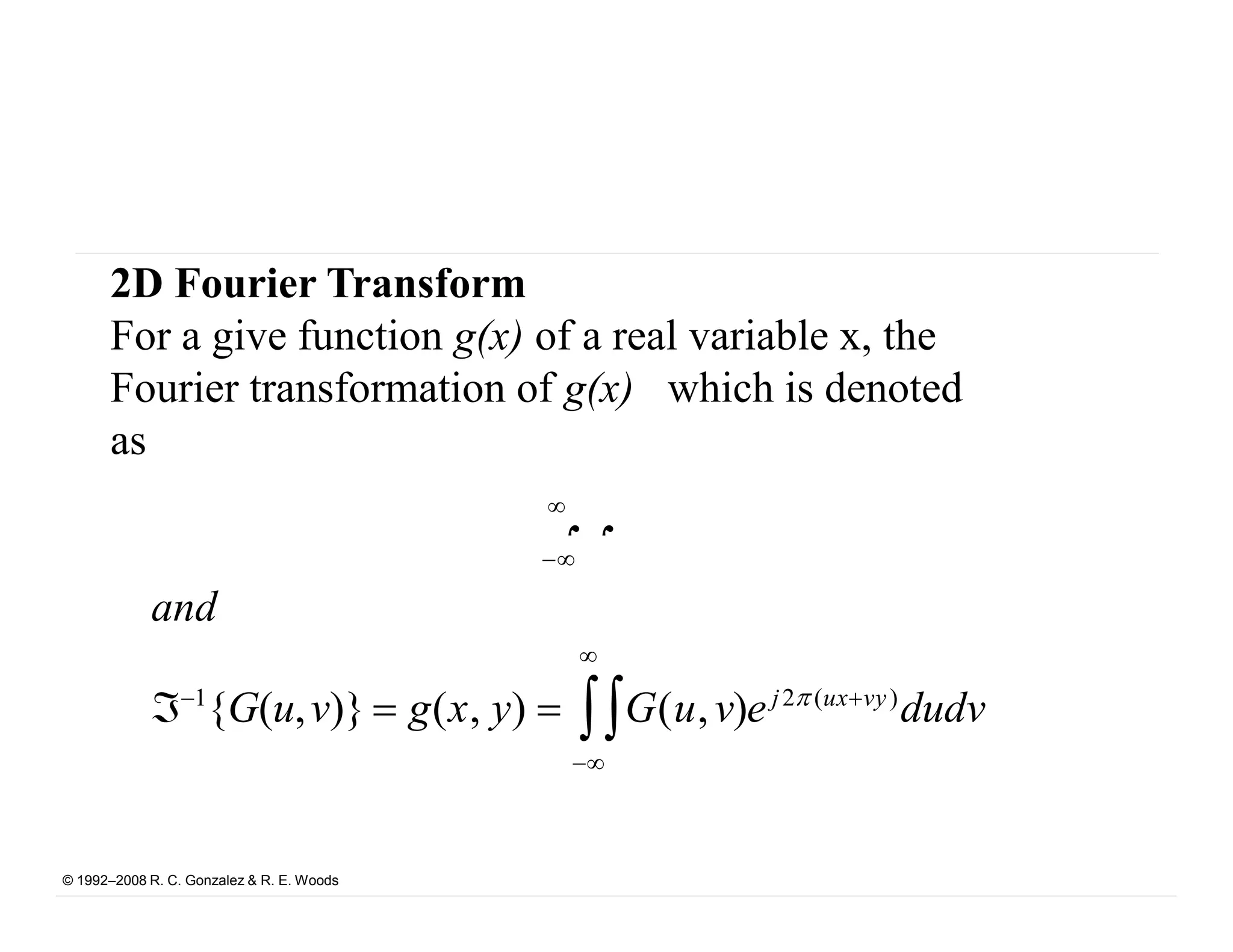
Step Function The unit step function, is a discontinuous function whose value is zero for negative argument and one for positive argument. A-A  t  0 0 t  0 H(t)  0 Rectangle Function The unit step function, is a discontinuous function whose value is zero for negative argument and one for positive argument. 0 t  A  A t  A Rect(t)   1 A-A  t A0 Impulse Function The Dirac delta function, or δ function, is zero for all values of the parameter except when the parameter is zero, and its integral over the parameter from −∞ to ∞ is equal to one  0 t 0 t 0 (t)   (t)dt 1  © 1992–2008 R. C. Gonzalez & R. E. Woods

Fourier Transform For a give function g(x) of a real variable x, the Fourier transformation of g(x) which is denoted as   j2ux - {g(x)} G(u) g(x)e dx   - 1 {g(x)} G(u) g(x)e dxj2ux Second Video

Since e j2t  sin(2t) jcos(2t) For that reason the Fourier transform F(u) F(u) = R(u) + jI(u) Which often appear as F(u) | F(u) | e j(u) | F(u) | R(u)2  I (u)2 R(u) © 1992–2008 R. C. Gonzalez & R. E. Woods tan( (u))  I(u)

. Spatial Domain Frequency Domain

2D Fourier Transform For a give function g(x) of a real variable x, the Fourier transformation of g(x) which is denoted as  {g(x, y)}  G(u, v)    g(x, y)e j 2 (uxvy ) dxdy and  1 {G(u,v)}  g(x, y)  G(u,v)ej2 (uxvy) dudv  © 1992–2008 R. C. Gonzalez & R. E. Woods

    AA X 0  1]   0  vY

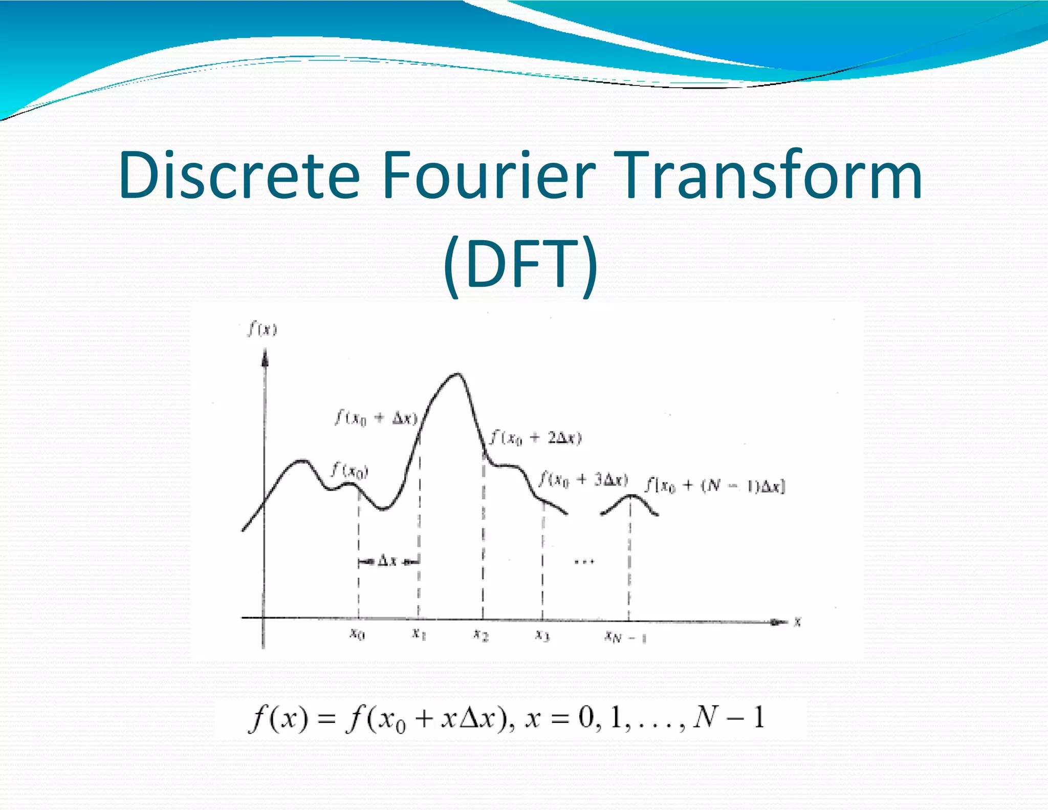
Discrete Fourier Transform •Let us discretize a continuous function f(x) into the N uniform samples that generate the sequence f(x0), f(x0+Δx), f(x0+2Δx), f(x0+3Δx), …, f(x0+[N-1]Δx) •Hence f(x) = f(x0+i Δx) •We could denote the samples as f(0), f(1), f(2), …,f(N-1). x0 and 0,1,2,..., N 1 N 1 1  f(x)e j 2ux / N ;u N • The Fourier Transform is F (u) N1 Third Video - Examples f (x)  F(u)e j2ux/ N u0

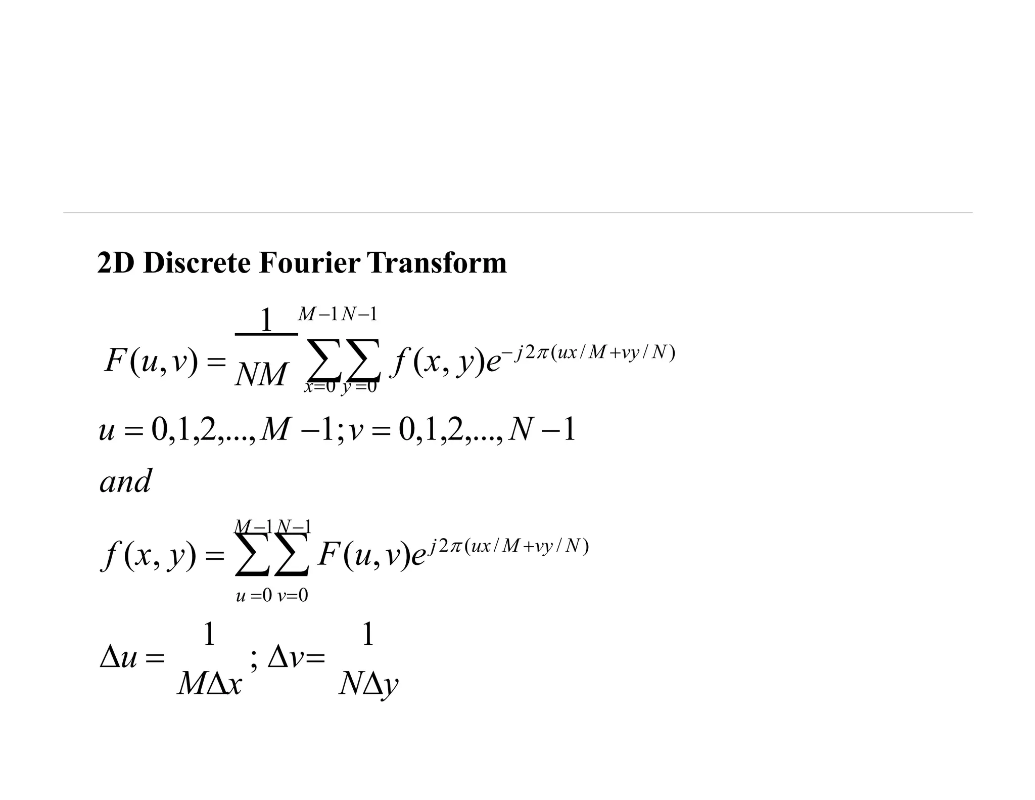
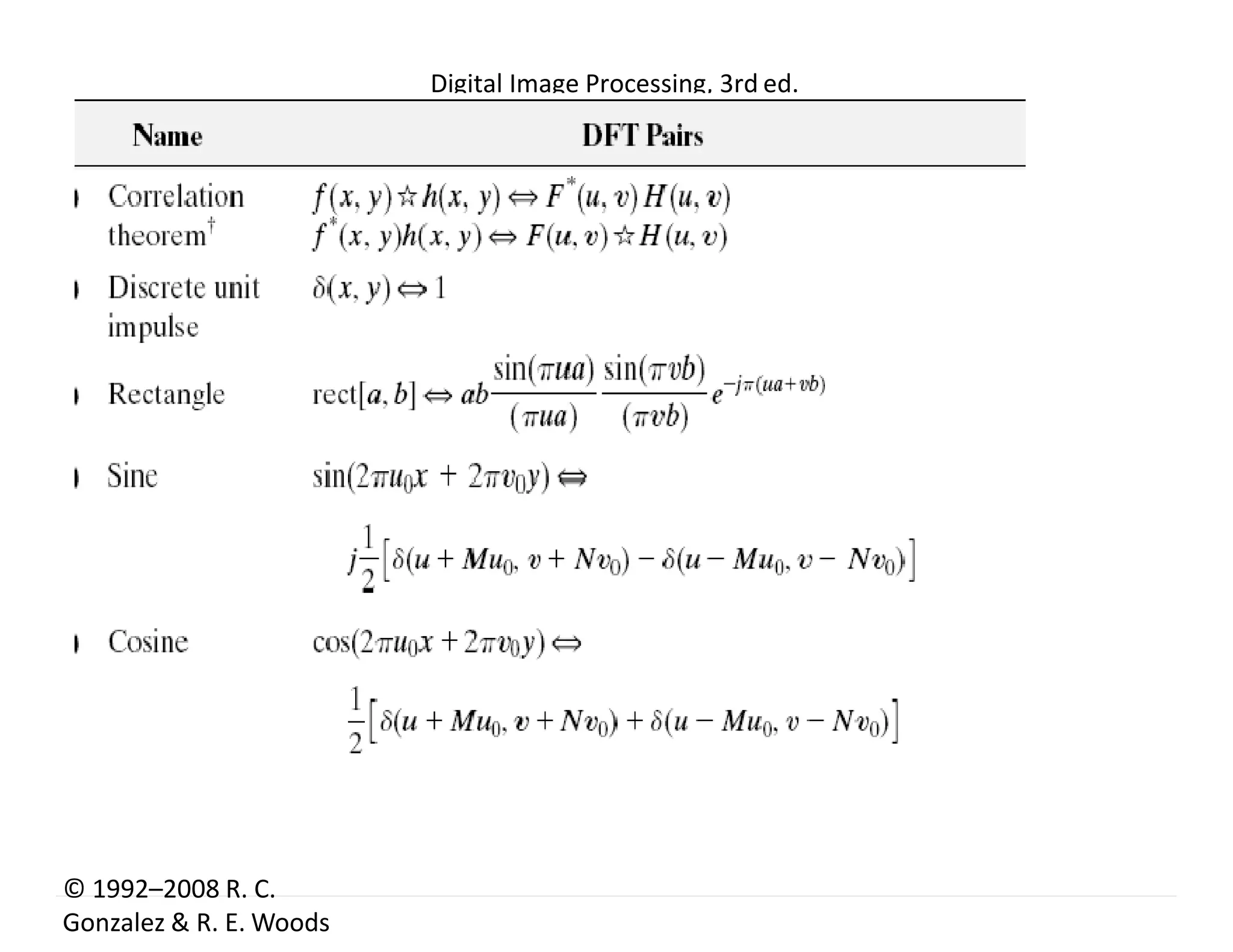
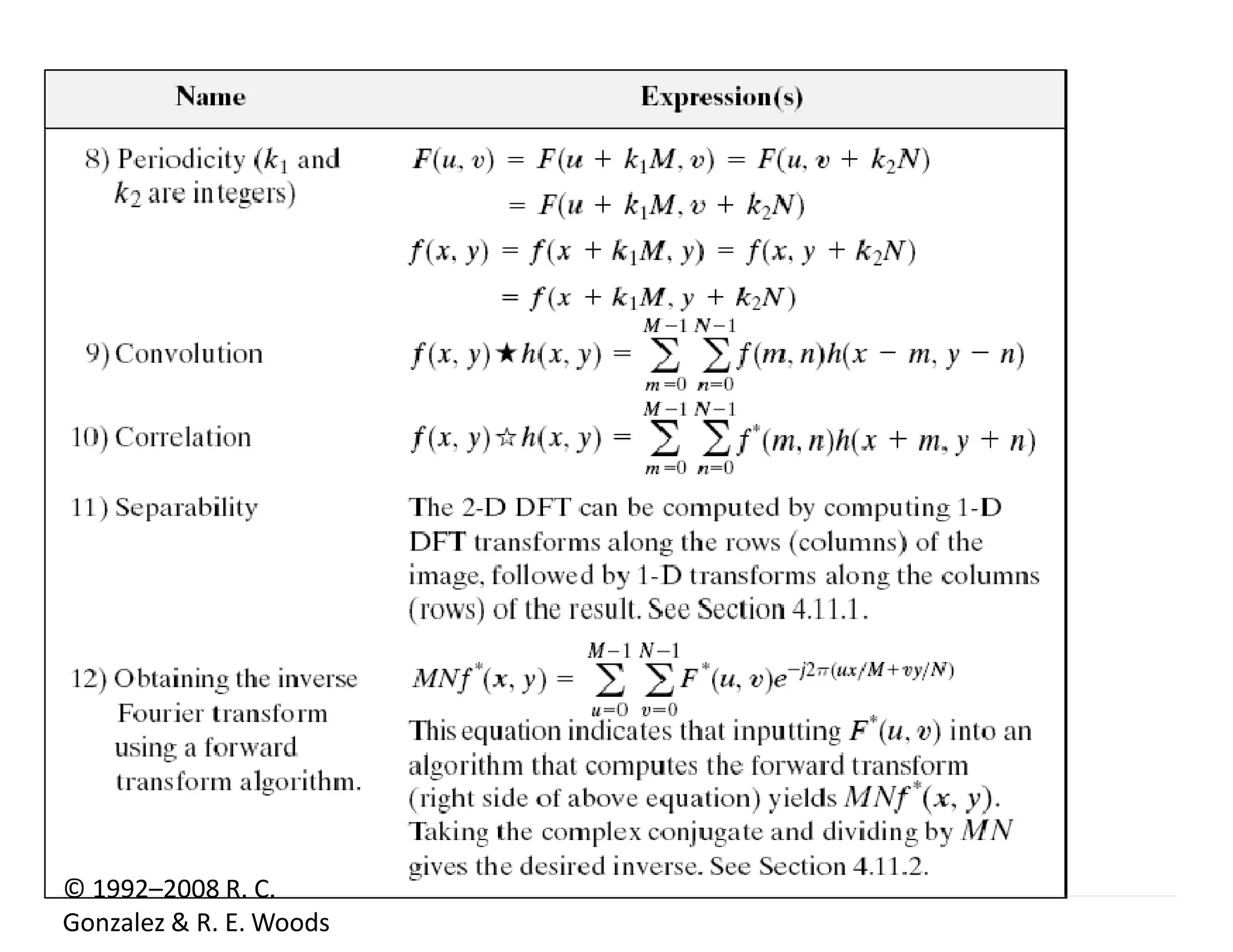
NM 2D Discrete Fourier Transform 1 M 1N 1 F(u,v)   f (x, y)e j2 (ux/ M vy / N ) x0 y 0 u  0,1,2,...,M 1;v  0,1,2,...,N 1 and M 1N1 1 1 f (x, y)   F(u,v)ej2 (ux/ M vy / N ) u 0 v0 Mx Ny u  ; v

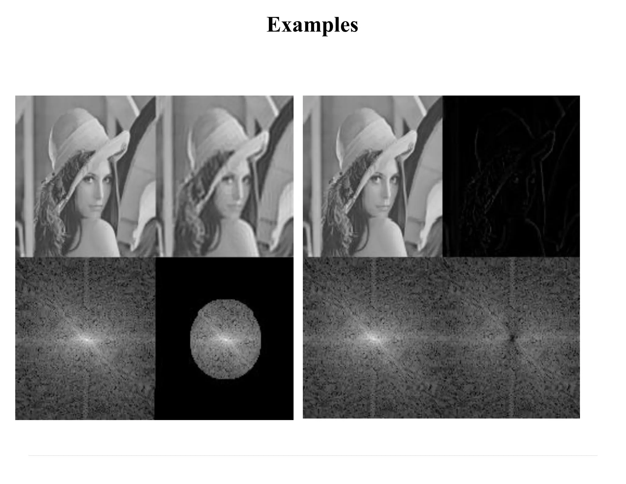
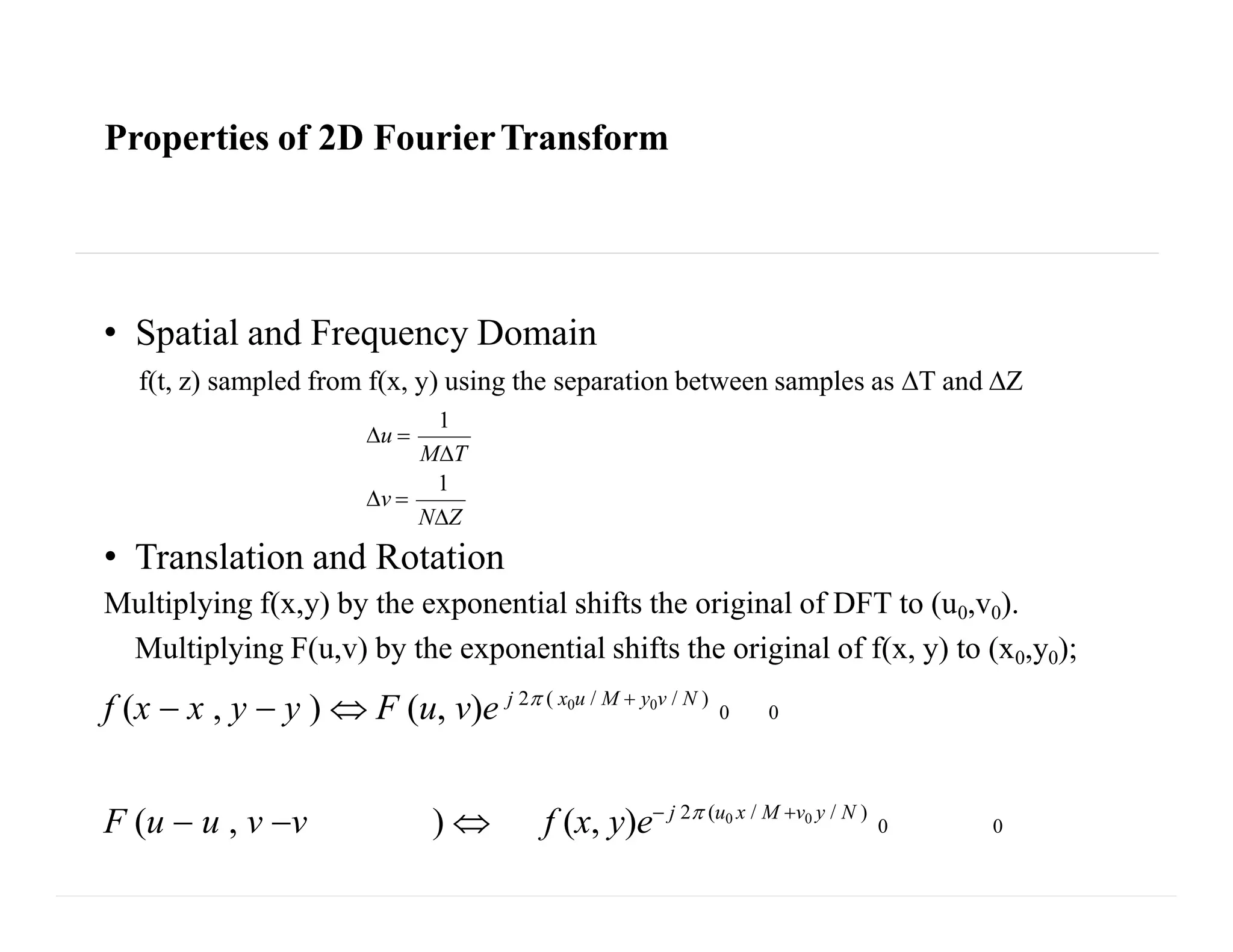
Properties of 2D FourierTransform • Spatial and Frequency Domain f(t, z) sampled from f(x, y) using the separation between samples as T and Z NZ v  MT 1 u  1 • Translation and Rotation Multiplying f(x,y) by the exponential shifts the original of DFT to (u0,v0). Multiplying F(u,v) by the exponential shifts the original of f(x, y) to (x0,y0); f (x  x , y  y )  F (u, v)e j 2 ( x0u / M  y0v / N ) 0 0 F (u  u , v v )  f (x, y)e j 2 (u0 x / M v0 y / N ) 0 0

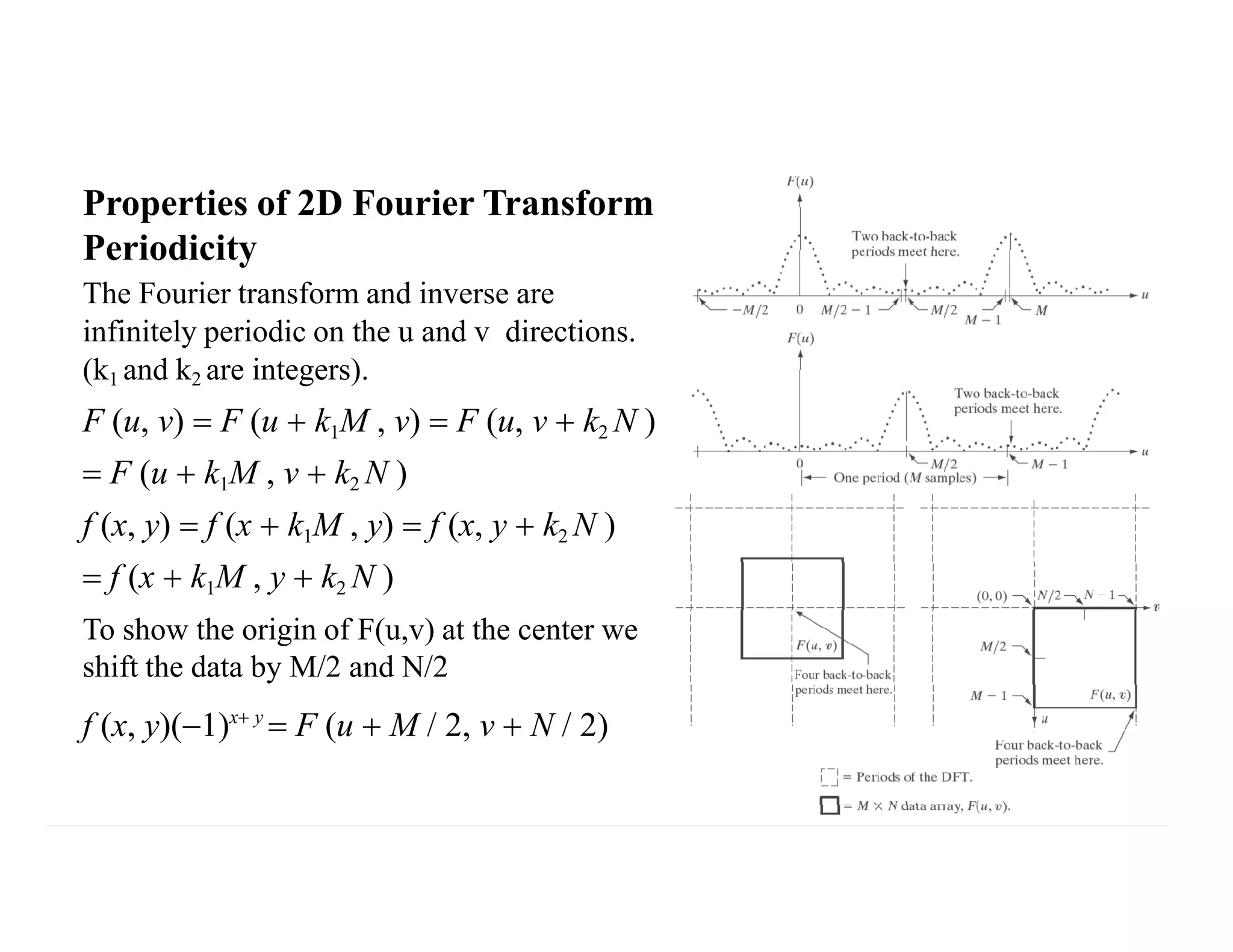
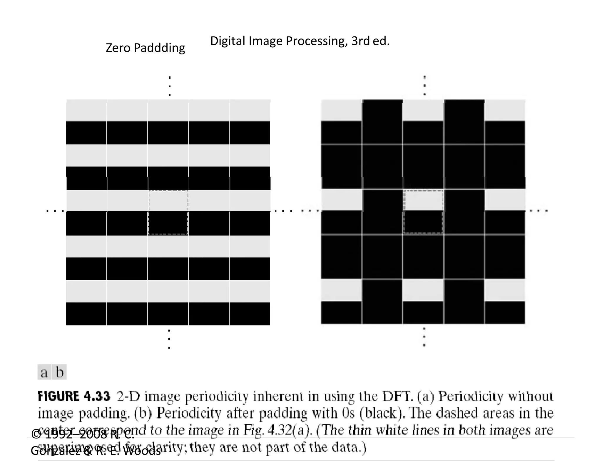
Properties of 2D Fourier Transform Periodicity The Fourier transform and inverse are infinitely periodic on the u and v directions. (k1 and k2 are integers). F (u, v)  F (u  k1M , v)  F (u, v  k2 N )  F (u  k1M , v  k2 N ) f (x, y)  f (x  k1M , y)  f (x, y  k2 N )  f (x  k1M , y  k2 N ) To show the origin of F(u,v) at the center we shift the data by M/2 and N/2 f (x, y)(1)x y  F (u  M / 2, v  N / 2)

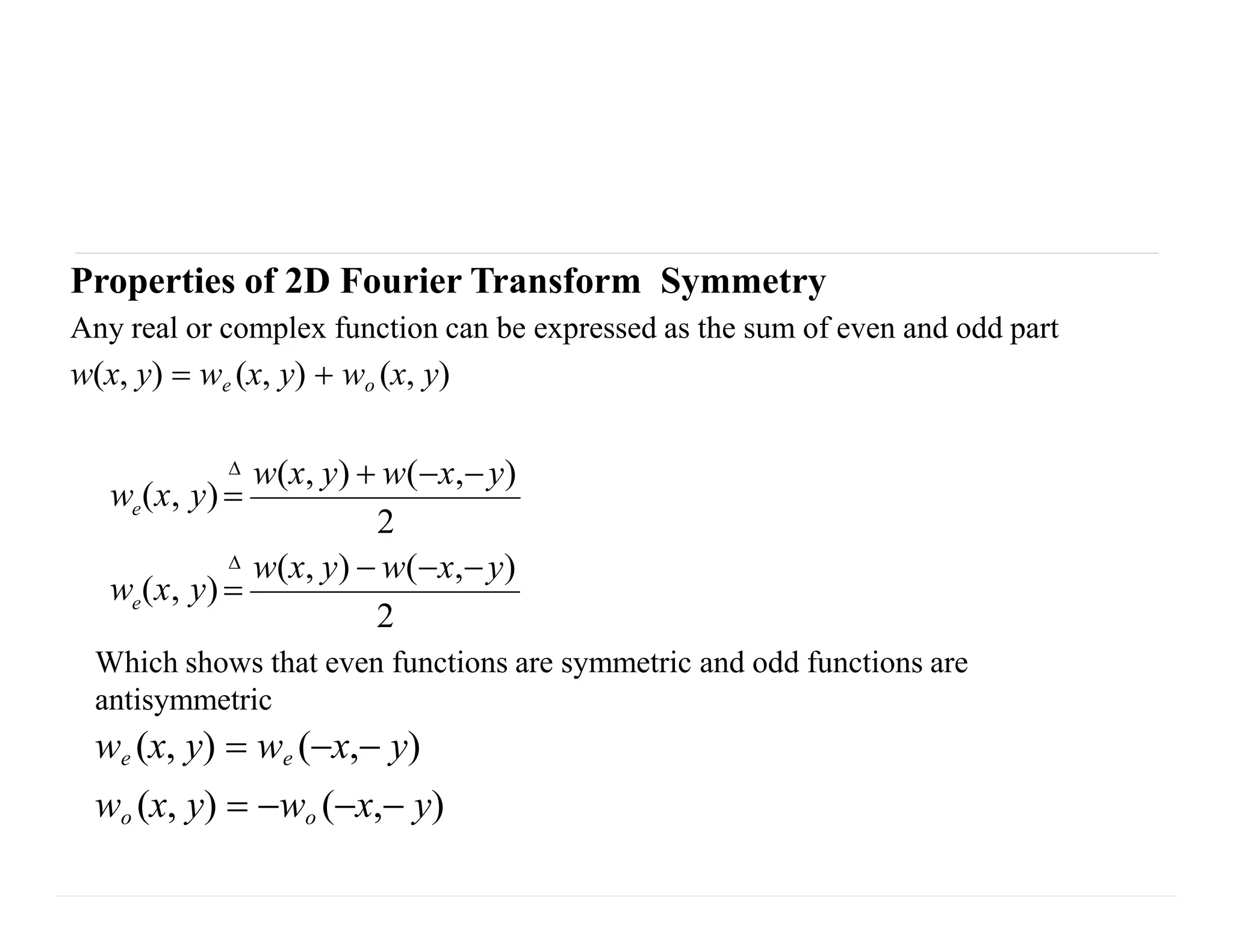
Properties of 2D Fourier Transform Symmetry Any real or complex function can be expressed as the sum of even and odd part w(x, y)  we (x, y)  wo (x, y) 2 w(x, y)  w(x,y) ew (x, y)  2 e w(x, y)  w(x,y) w (x, y)   Which shows that even functions are symmetric and odd functions are antisymmetric we (x, y)  we (x, y) wo (x, y)  wo (x, y)

Properties of 2D Fourier Transform Symmetry The Fourier transform of a real function f(x,y) is conjugate symmetric F* (u,v)  F(u,v) The Fourier transform of a imaginary function f(x,y) is conjugate anti-symmetric F* (u,v)  F(u,v) 1  * x0 y 0NM   F* (u,v)   M 1N1  f (x, y)e j2 (ux / M vy/ N ) Proof NM x0 y 0 1 N1  1 M  f * (x, y)ej2 (ux/ M vy/ N ) 1 N1  1 M  f (x, y)e j2 ([u]x/ M [v]y / N ) NM  F(u,v) x0 y 0

Sampling and Fourier Transform 1.Converting continuous function/signal into a discrete one. 2.The sampling is uniform at T intervals The sampled function and the value of each Sample are : ~ f (t)f (t)  f (t)s (t)    (t  nT)T n  fk   f (t) (t  kT )dt  f (kT) 

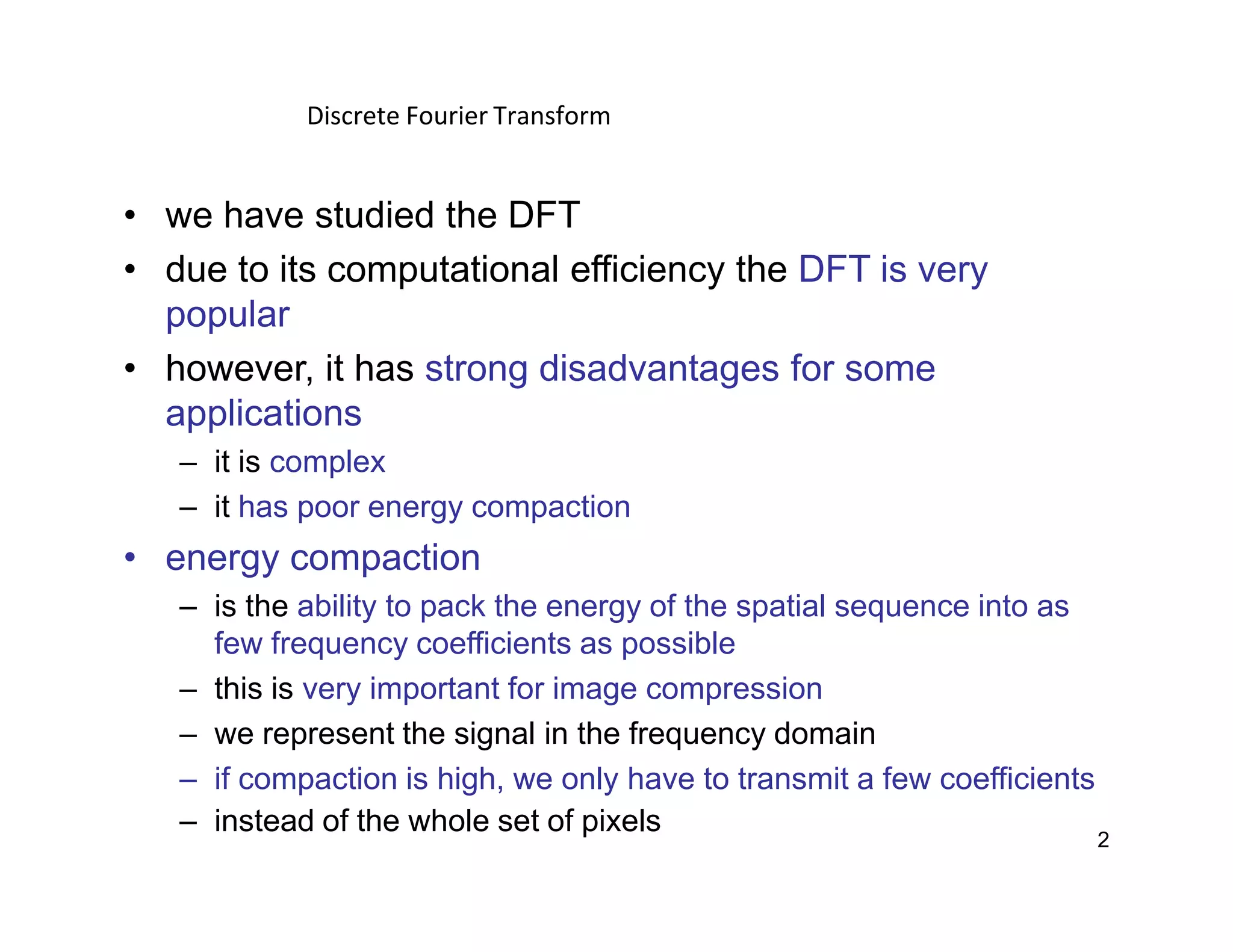
Sampling Theorem Band limited-A function f(t) whose Fourier transform is zero out of the interval [-max , max] is called band limited ~ We can recover a function f(t) from its sampled representation if we can isolate a copy of F() from the periodic sequence of copies. Extracting from F() a single period that represents F() is possible in the separation between copies is sufficient , which is guaranteed if ½T > max max 2 1 T Which is call the Nyquist Rate © 1992–2008 R. C. Gonzalez & R. E. Woods

. Application of Filters H(U,V)

Discrete Fourier Transform 2 • we have studied the DFT • due to its computational efficiency the DFT is very popular • however, it has strong disadvantages for some applications – it is complex – it has poor energy compaction • energy compaction – is the ability to pack the energy of the spatial sequence into as few frequency coefficients as possible – this is very important for image compression – we represent the signal in the frequency domain – if compaction is high, we only have to transmit a few coefficients – instead of the whole set of pixels

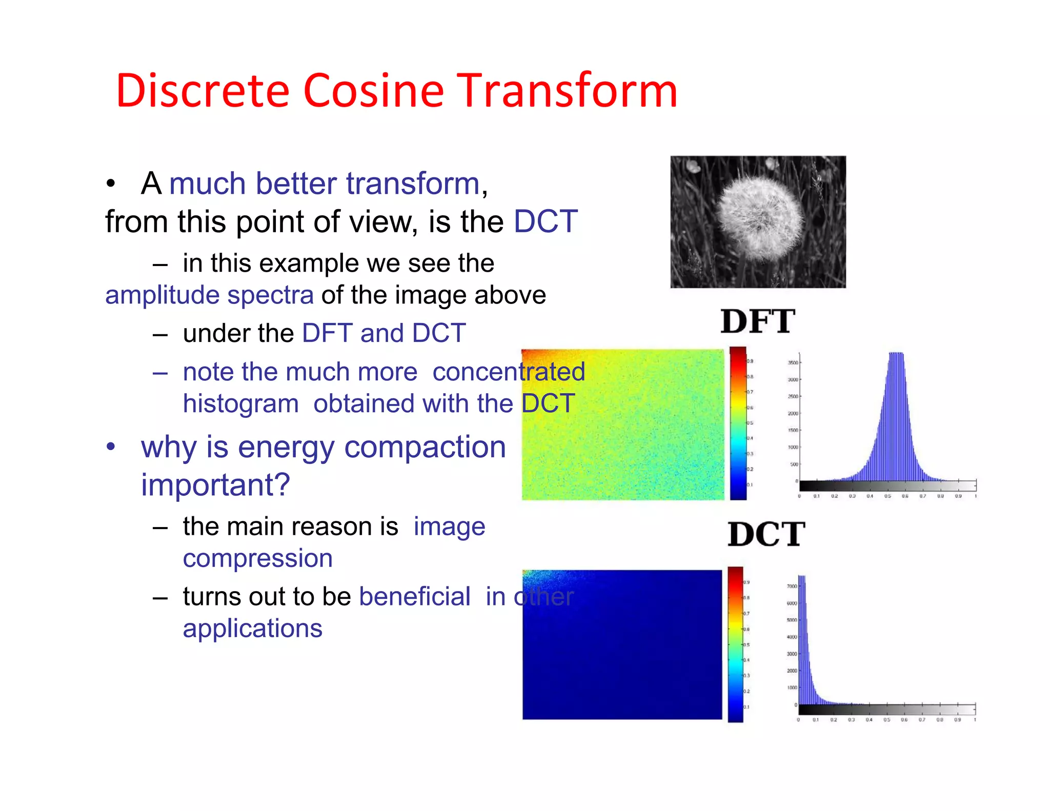
Discrete Cosine Transform • A much better transform, from this point of view, is the DCT – in this example we see the amplitude spectra of the image above – under the DFT and DCT – note the much more concentrated histogram obtained with the DCT • why is energy compaction important? – the main reason is image compression – turns out to be beneficial in other applications 3

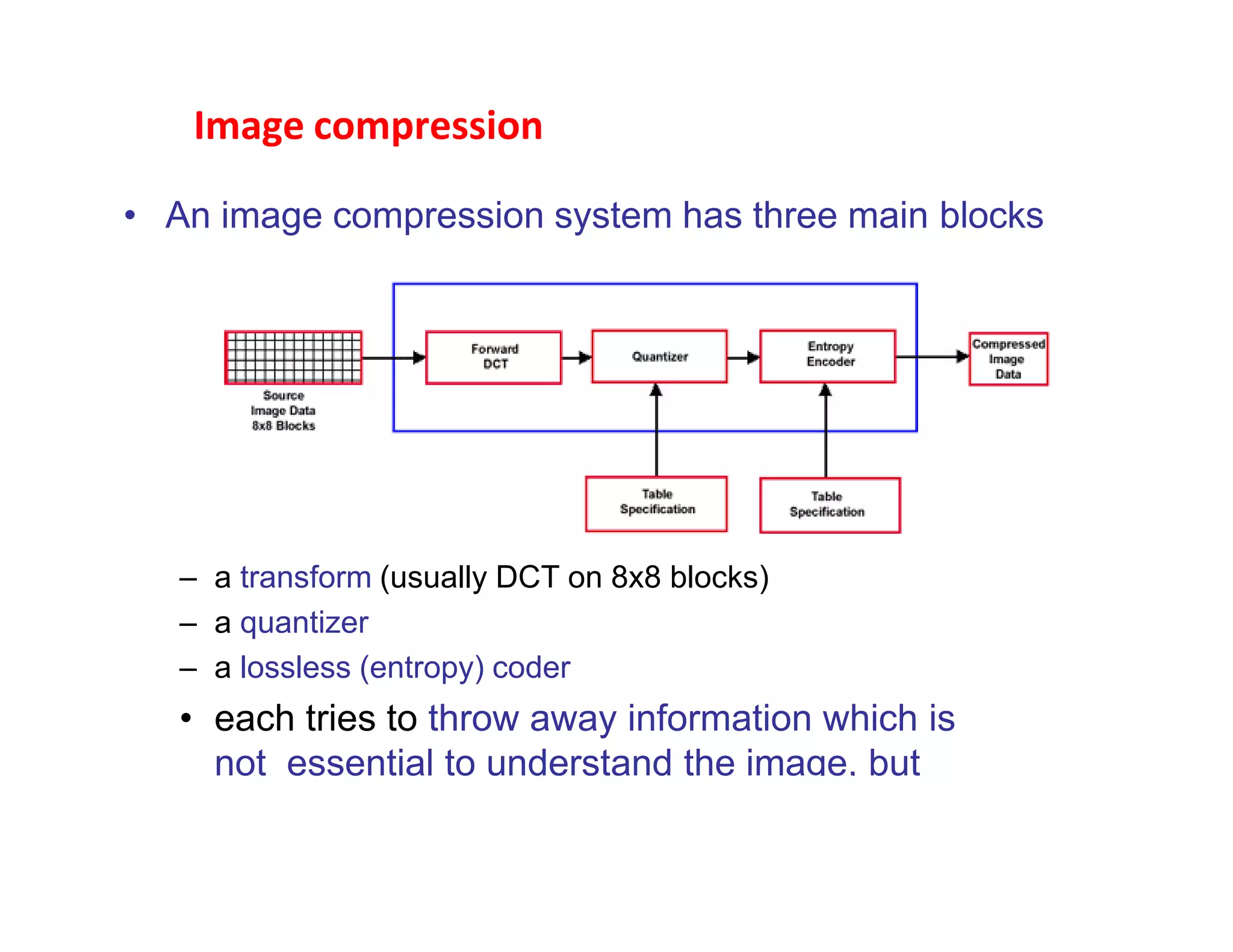
Image compression • An image compression system has three main blocks – a transform (usually DCT on 8x8 blocks) – a quantizer – a lossless (entropy) coder • each tries to throw away information which is not essential to understand the image, but costs bits

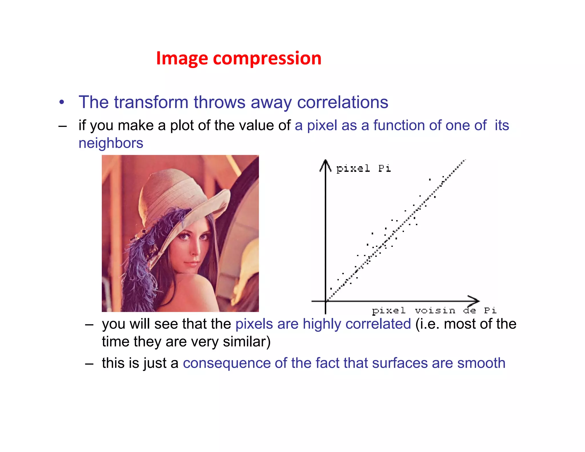
• The transform throws away correlations – if you make a plot of the value of a pixel as a function of one of its neighbors – you will see that the pixels are highly correlated (i.e. most of the time they are very similar) – this is just a consequence of the fact that surfaces are smooth Image compression

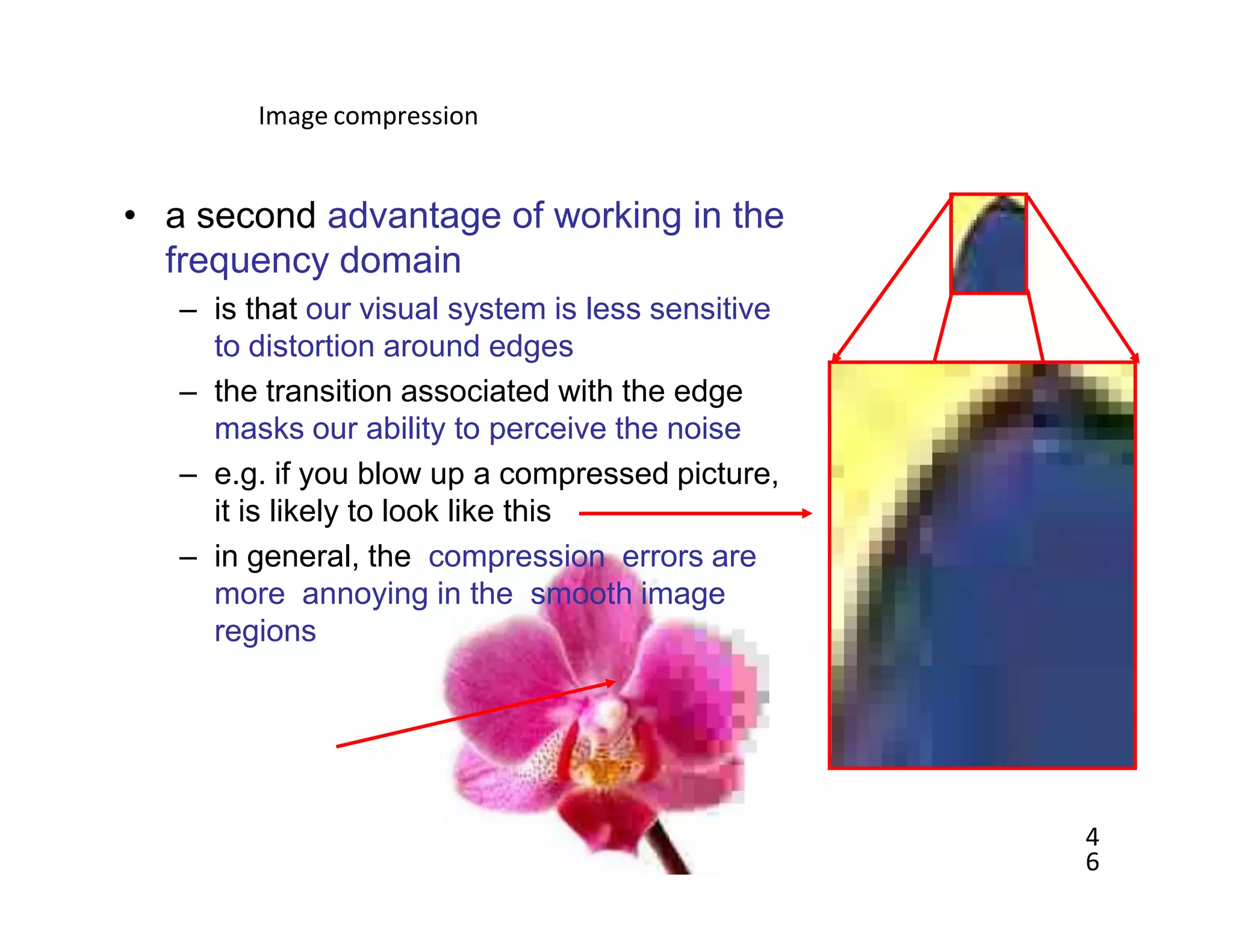
Image compression • a second advantage of working in the frequency domain – is that our visual system is less sensitive to distortion around edges – the transition associated with the edge masks our ability to perceive the noise – e.g. if you blow up a compressed picture, it is likely to look like this – in general, the compression errors are more annoying in the smooth image regions 4 6

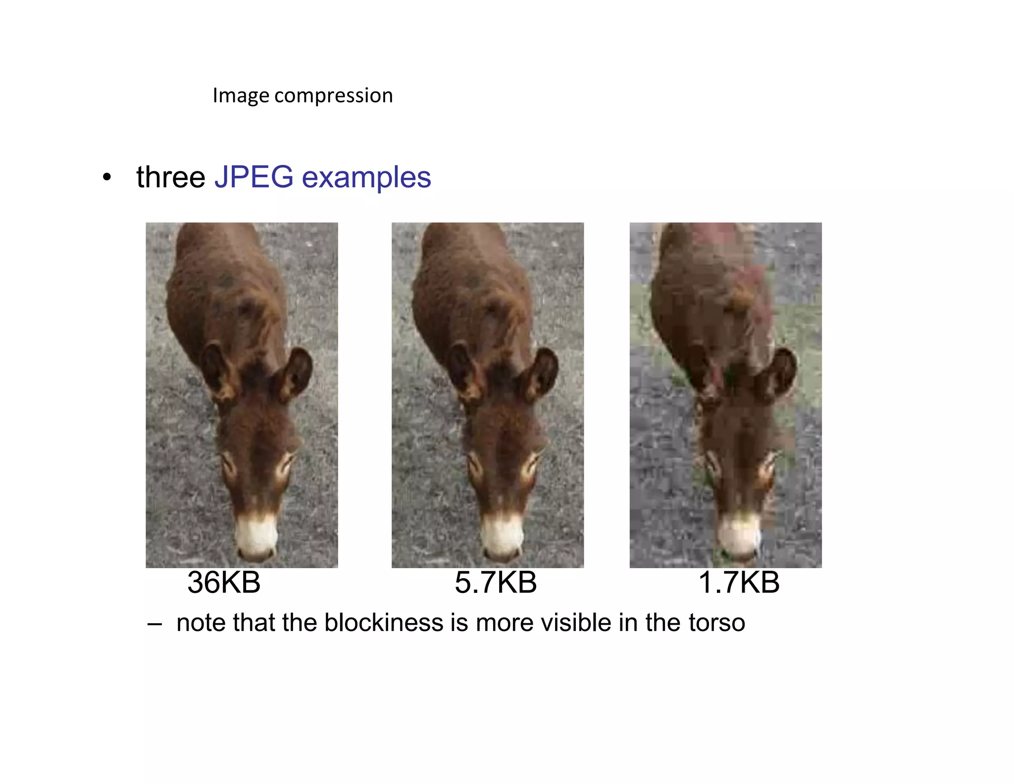
Image compression • three JPEG examples 36KB 5.7KB 1.7KB – note that the blockiness is more visible in the torso

Image compression • important point: – does not save any bits – does not introduce any distortion • both of these happen when we throw away information • this is called “lossy compression” and implemented by the quantizer • what is a quantizer? – think of the round() function, that rounds to the nearest integer – round(1) = 1; round(0.55543) = 1; round (0.0000005) = 0 – instead of an infinite range between 0 and 1 (infinite number of bits to transmit) – the output is zero or one (1 bit) – we threw away all the stuff in between, but saved a lot of bits – a quantizer does this less drastically

Quantizer • it is a function of this type – inputs in a given range are mapped to the same output • to implement this, we – 1) define a quantizer step size Q – 2) apply a rounding function  x    Q x  roundq – the larger the Q, the less reconstruction levels we have – more compression at the cost of larger distortion – e.g. for x in [0,255], we need 8 bits and have 256 color values – 4 levels and only need 2 bits

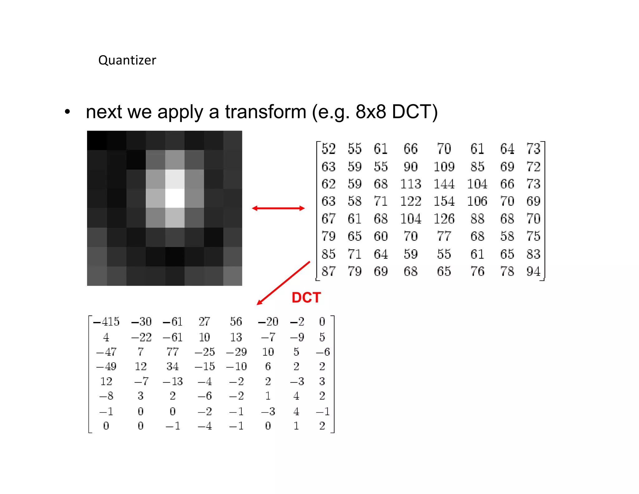
Quantizer • note that we can quantize some frequency coefficients more heavily than others by simply increasing Q • this leads to the idea of a quantization matrix • we start with an image block (e.g. 8x8 pixels)

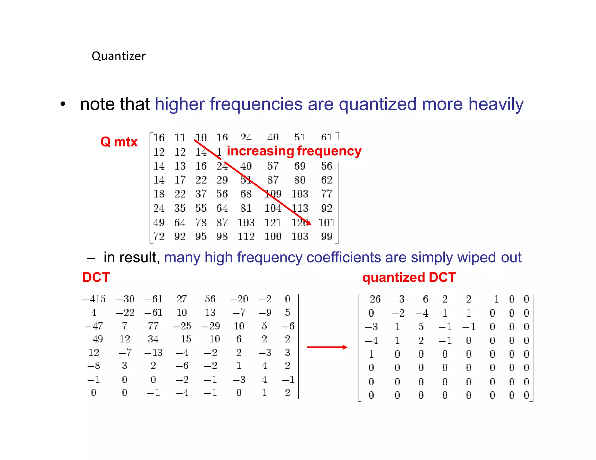
Quantizer • next we apply a transform (e.g. 8x8 DCT) DCT

Quantizer • and quantize with a varying Q DCT Q mtx

Quantizer • note that higher frequencies are quantized more heavily Q mtx increasing frequency – in result, many high frequency coefficients are simply wiped out DCT quantized DCT

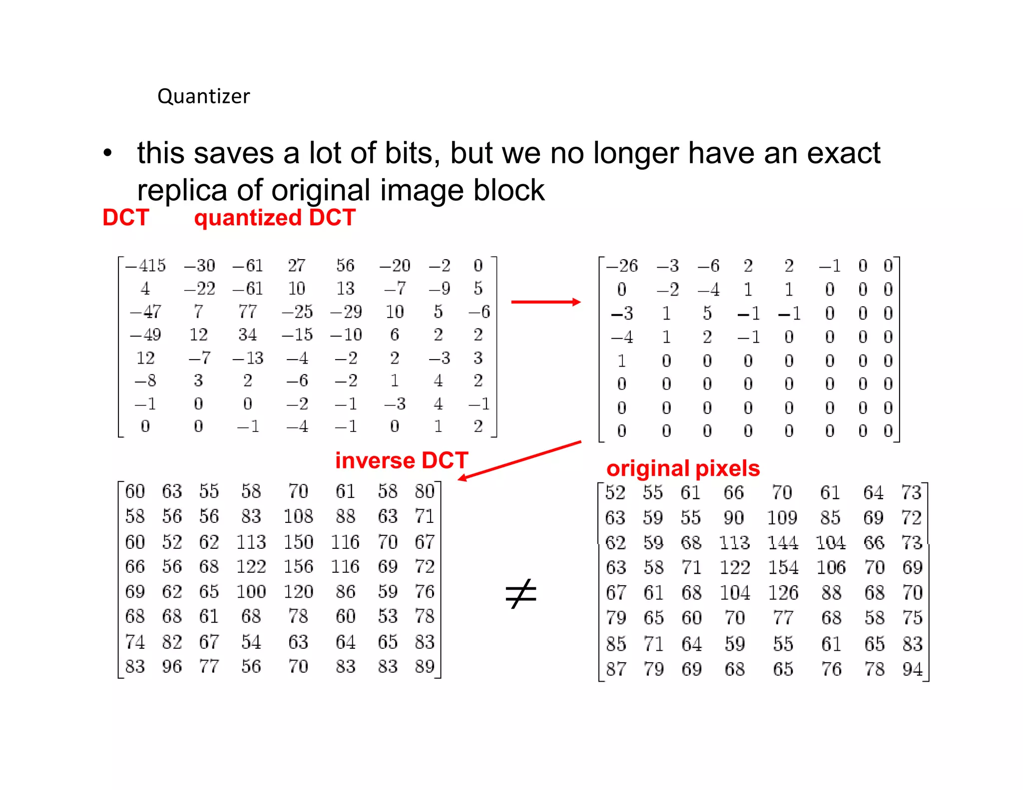
Quantizer • this saves a lot of bits, but we no longer have an exact replica of original image block DCT quantized DCT inverse DCT original pixels 

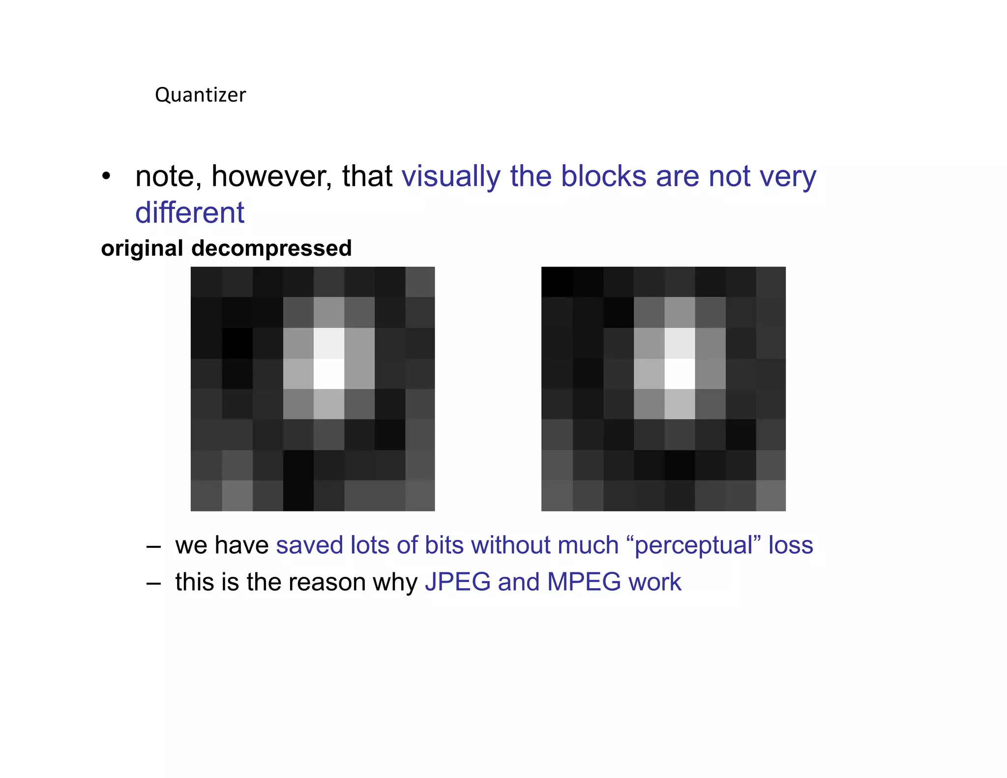
Quantizer • note, however, that visually the blocks are not very different original decompressed – we have saved lots of bits without much “perceptual” loss – this is the reason why JPEG and MPEG work

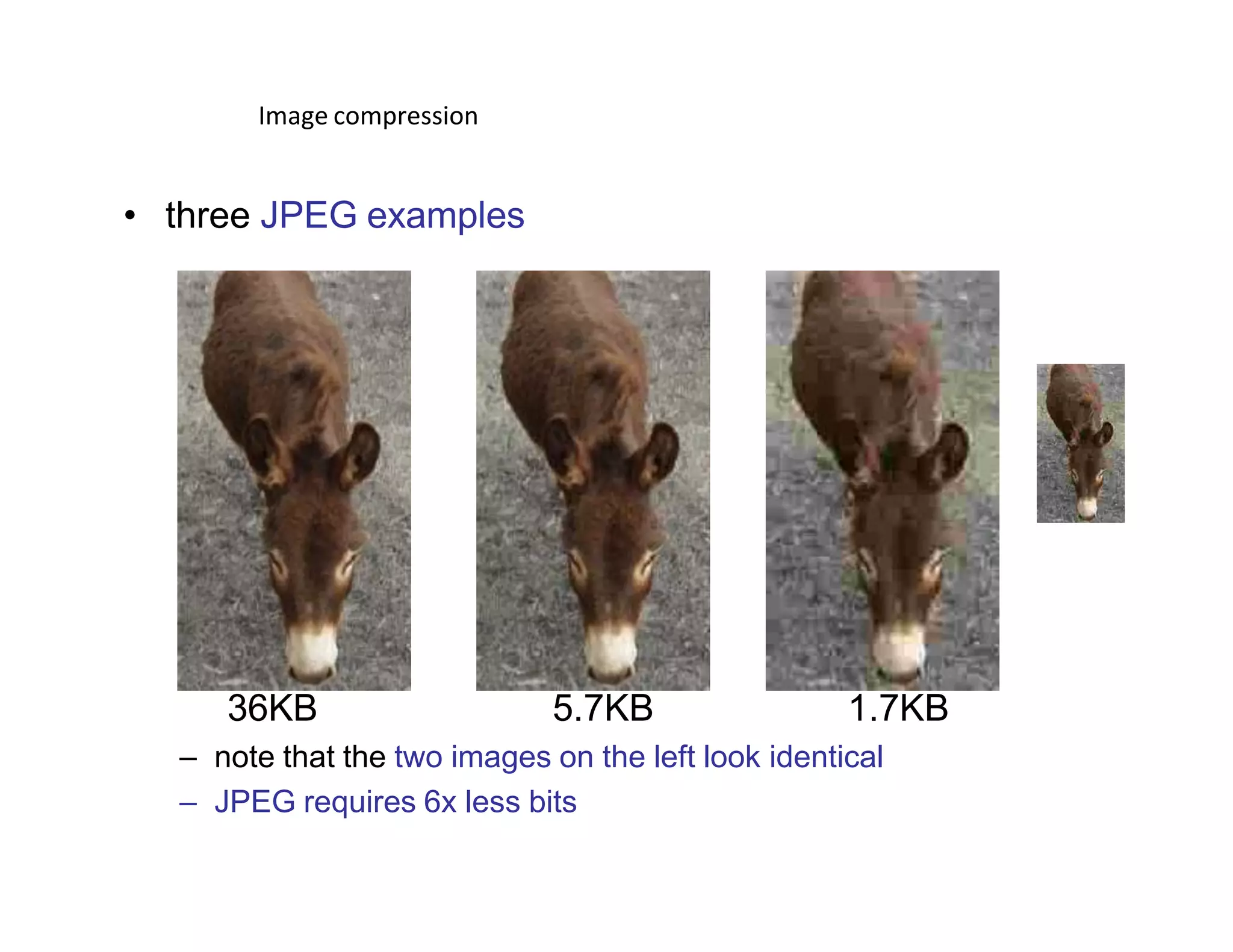
Image compression • three JPEG examples 36KB 5.7KB 1.7KB – note that the two images on the left look identical – JPEG requires 6x less bits

Energy compaction • The two extensions are DFT DCT – note that in the DFT case the extension introduces discontinuities – this does not happen for the DCT, due to the symmetry of y[n] – the elimination of this artificial discontinuity, which contains a lot of high frequencies, – is the reason why the DCT is much more efficient

2D-DCT n2n2 1D-DCT • 1) create intermediate sequence by computing 1D-DCT of rows • 2) compute k1 f [ k1 , n 2 ] n1 x[ n1 , n 2 ] 1D-DCT of columns n2 k2 1D-DCT k1 f [ k 1 , n 2 ] 5 8 k1 C x [ k 1 , k 2 ] • the extension to 2D is trivial • the procedure is the same

DIGITAL IMAGE PROCESSING - Day 4 Image Transform

In this document

More Related Content

What's hot

Similar to DIGITAL IMAGE PROCESSING - Day 4 Image Transform

More from vijayanand Kandaswamy

Recently uploaded

DIGITAL IMAGE PROCESSING - Day 4 Image Transform