![Page | 703 © 2013, Hindawi All Rights Reserved Volume 2013 Journal of Electrical and Computer Engineering Research Paper Available online at: www.hindawi.com Efficient Block Classification of Computer Screen Images for Desktop Sharing using Neural Network P.S.Jagadeesh Kumar Department of Computer Science University of Cambridge, United Kingdom Abstract— This paper presents a neural network based efficient block classification of compound images for desktop sharing. The objective is to maximize the precision and recall rate of the classification algorithm, while at the same time minimizing the execution and training time of the neural network. It segments computer screen images into text/graphics, picture/background blocks by using as input, the statistical features based on DWT coefficients in the sub-bands of each 8×8 block. The proposed algorithm can perform accurate block classification of text information with different fonts, sizes and ways of arrangement from the background image, so that text/graphics blocks can be compressed at higher quality than background image blocks. The proposed work is expected to minimize block classification error due to the adaptive nature of neural network. Keywords— Compound image, Neural Network, Block Classification, Segmentation I. INTRODUCTION A picture can say more than a thousand words. Unfortunately, storing an image can cost more than a million words. This isn't always a problem, because many of today's computers are sophisticated enough to handle large amounts of data. Sometimes however you want to use the limited resources more efficiently. Digital cameras for instance often have a totally unsatisfactory amount of memory, and the internet can be very slow. Mostly in internet, it is necessary to send the digital type of images using digital camera, personal computers. It contains more and more compound images. While sending the compound images, it occupies more size and takes large amount of time to attach. In such conditions, compound image compression is needed and thus requires rethinking of our approach to compression. In this paper, the block based segmentation approach is considered and it gives the better result. In the case of object based approach, complexity is the main drawback, since image segmentation may require the use of very sophisticated segmentation algorithms. In layer based segmentation, the main drawbacks are mismatch between the compression method and the data types, and an intrinsic redundancy due to the fact that the same parts of the original image appear in several layers. But in the block based segmentation it gives the better mismatch between the region boundaries and the compression algorithms, and the lack of redundancy. The proposed block classification algorithm has low calculation complexity, which makes it very suitable for real-time application. II. SEGMENTATION The proposed compound image compression for real-time computer screen image transmission follows first- pass of two-pass segmentation procedure and classifies image blocks into picture and text/graphics blocks by thresholding the number of colors of each block. Basic shape primitives of text/graphics from picture blocks, shape primitives from text/graphics blocks are extracted and are lossless coded using a combined shape-based and palette based coding algorithm. Pictorial blocks are coded by lossy JPEG [1, 2]. So numerous coding algorithms are needed in this method and basic shape primitives defined in this method is not ample for text of different sizes. In this paper, the proposed algorithm first classifies 8 × 8 non-overlapping blocks of pixels into two classes, such as, text/graphics and picture/background based on the statistical feature computed from detail sub-band coefficients of each 8 × 8 DWT transformed image block [3, 6]. Then, each class is compressed using an algorithm specifically designed for that class. The proposed one-pass block classification simplifies segmentation by separating the image into two classes of pixels and also minimizes misclassification error irrespective of font color, style, orientation and background complexity. III. WAVELET TRANSFORM Unlike the Fourier transform, whose basis functions are sinusoids, wavelet transforms are based on small waves called wavelets of varying frequency and limited duration. In 1987, wavelets are first shown to be the foundation of a powerful new approach to signal processing and analysis called multi-resolution theory. Multi-resolution theory incorporates and unifies techniques from a variety of disciplines including sub-band coding signal processing, quadrature mirror filtering from digital speech recognition and pyramidal image processing [4, 5]. Another important imaging technique with ties to multi-resolution analysis sub-band coding. In this coding, an image is decomposed into a set of band-limited components called sub-bands, which can be reassembled to reconstruct the original image without error.](https://image.slidesharecdn.com/efficientblockclassificationofcomputerscreenimagesfordesktopsharingusingneuralnetwork-210208072715/75/Efficient-Block-Classification-of-Computer-Screen-Images-for-Desktop-Sharing-using-Neural-Network-1-2048.jpg)
![Page | 711 © 2013, Hindawi All Rights Reserved PSJ Kumar, Journal of Electrical and Computer Engineering, 2013, pp. 703-711 Fig.16 Runtime for project in train mode using „ch1.jpg‟ REFERENCES [1] Florinabel D J, Juliet S E, Dr Sadasivam V, Efficient Coding of Computer Screen Images with Precise Block Classification using Wavelet Transform. Volume 91 May 2010. [2] Gonzalez R C, Woods R E and Eddins S L. „Digital Image Processing using MATLAB‟. Prentice Hall, Upper Saddle River, NJ, 2004. [3] Keslassy I, Kalman M, Wang D and Girod B. „Classification of Compound Images based on Transform Coefficient Likelihood‟. Proceedings of International Conference on Image Processing, vol 1, October 2001. [4] Mallat S. „A Wavelet Tour of Signal Processing‟. Second Edition, Academic Press, 1999. [5] A. Said and A. Drukarev, “Simplified segmentation for compound image compression”, Proceeding of ICIP‟ 2009, pp.229-233. [6] H. Cheng and C.A. Bouman, “Multiscale Bayesian segmentation using a trainable context model” IEEE Trans.Image Processing, vol. 10, pp. 511–525, April 2001.](https://image.slidesharecdn.com/efficientblockclassificationofcomputerscreenimagesfordesktopsharingusingneuralnetwork-210208072715/75/Efficient-Block-Classification-of-Computer-Screen-Images-for-Desktop-Sharing-using-Neural-Network-9-2048.jpg)

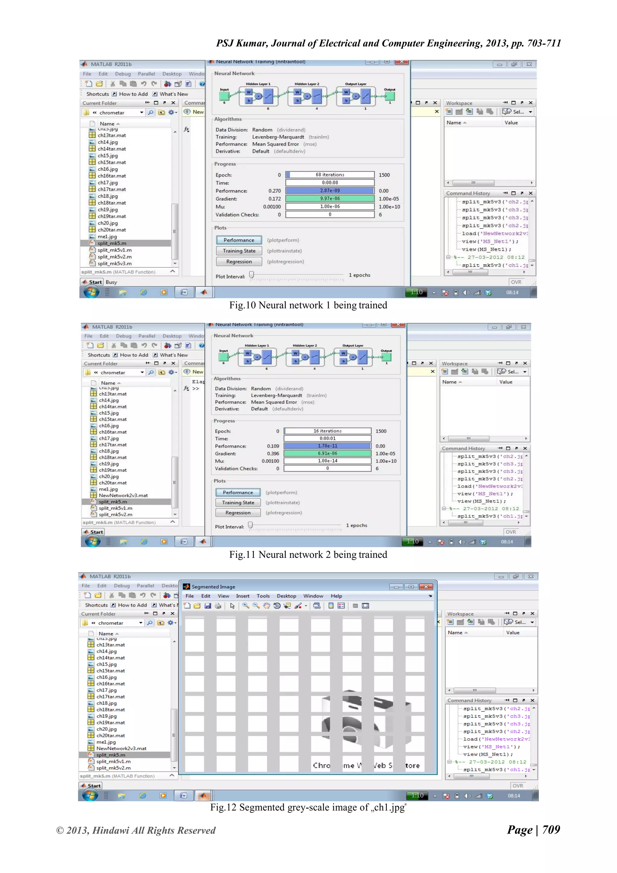
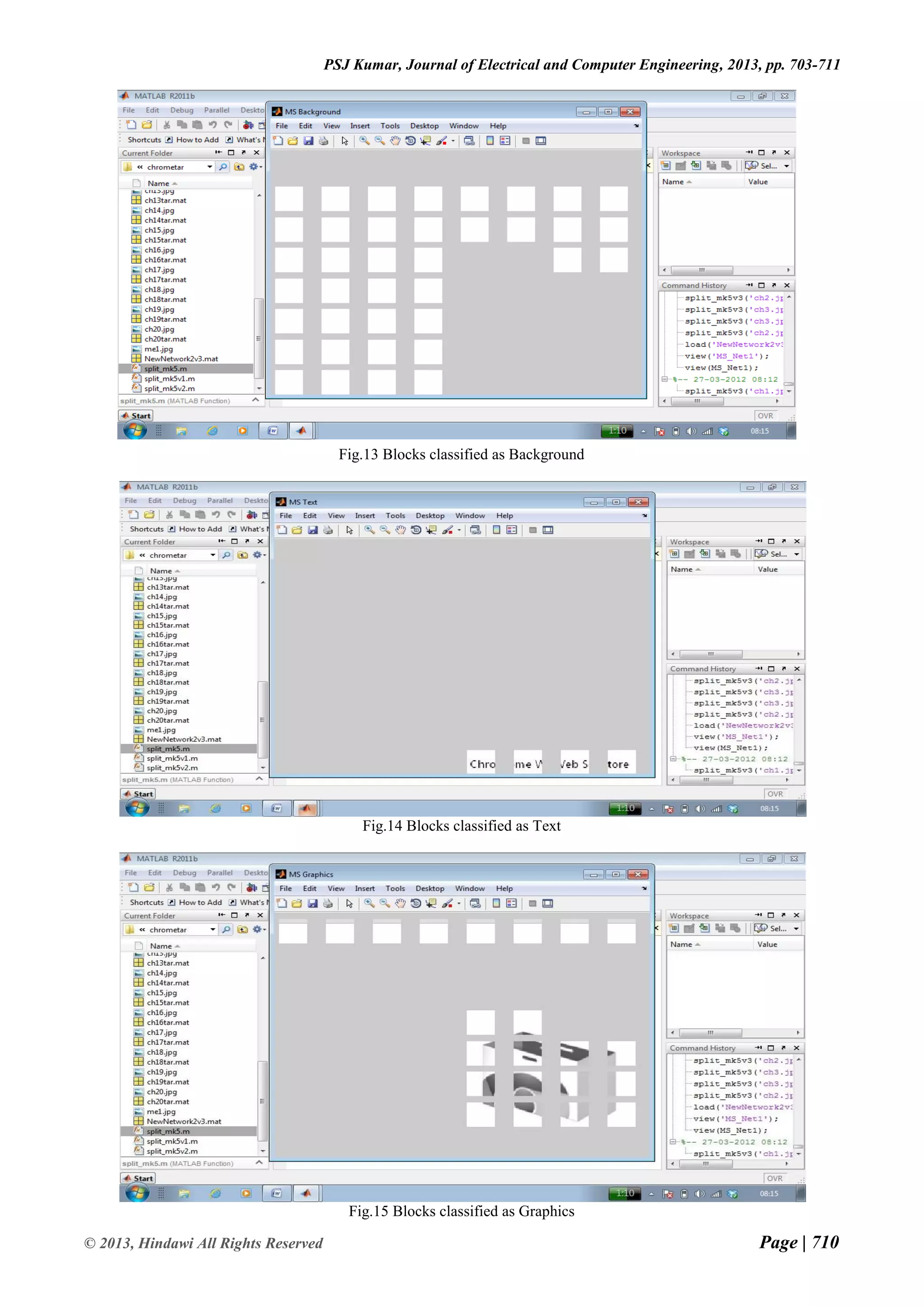
The document presents a neural network approach for efficient block classification of computer screen images for desktop sharing. It segments screen images into text/graphics and picture/background blocks using discrete wavelet transform coefficients and statistical features of 8x8 blocks. The neural network is trained to classify blocks into the two classes and minimize classification errors. Experimental results show the approach achieves over 95% accuracy on various test images with minimal training time and iterations. Future work could aim to further improve classification accuracy.