Finding Meaning in Points, Areas and Surfaces: Spatial Analysis in R

Finding Meaning in Points, Areas and Surfaces: Spatial Analysis in R Revolution Analytics Wednesday 13th June 1300 EST

The instructor • Dave Unwin • Retired Geography professor • University of London, UK • Spatial analysis & GIS in environmental sciences

Geography is everywhere? • Everything happens somewhere • Interest is on geo-spatial data at scales from a few meters to the planet Earth

Spatial analysis is the name given to a variety of methods of analysis in which we use LOCATION as an explanatory variable NB: Not all spatial analysis is spatial statistical analysis and not all spatial analysis is geospatial

Typical Questions • Is there an unusual clustering of point objects such as crimes/cases of a disease/trees/whatever here that we need to worry about? If so does the point pattern help explain why? • Does this phenomenon in these areas (counties, states, countries) show spatial variation I need to know about? Does the pattern help explain why? • What is the most probable value for a continuous variable at this location?

Characteristics of spatial data? • Almost always given: typically the analyst has no choice in their acquisition, sometimes even their formatting; • They have additional structure that defines their geometry (point, line/network, area/lattice, surface/field/geostatistical)

Types of spatial data Objects can be points, lines/networks or areas/lattices with L0, L1 and L2 dimension of length Fields are self-defining and spatially continuous: everywhere has a value (e.g. temperature, mean annual rainfall, …)

Locating things on Planet Earth • There are many ways by which we measure our location (place name, address, ZIP/Post code , latitude/longitude, grid reference etc) • How we locate depends on context and scale • Spatial resolution of location measurements vary • For analysis we (usually) need (x, y) co-ordinates in a projected system • Need for keys to provide these data, often added after the data have been collected • GPS & GPS-enabled devices are changing this and LBS is a massive and growing industry that is changing our spatial behaviour

Why R? • A consistent environment for statistical computing and graphics • Relative proximity to the data • Easy links to code in numerous languages and to DBMS • Easier development of new methods • Packages available to perform most analyses • Immensely supportive community

The sp Spatial Class and its subclasses

> library(sp) > getClass("Spatial") Class "Spatial" [package "sp"] Slots: Name: bbox proj4string Class: matrix CRS Known Subclasses: Class "SpatialPoints", directly Class "SpatialLines", directly Class "SpatialPolygons", directly Class "SpatialPointsDataFrame", by class "SpatialPoints", distance 2 Class "SpatialPixels", by class "SpatialPoints", distance 2 Class "SpatialLinesDataFrame", by class "SpatialLines", distance 2 Class "SpatialGrid", by class "SpatialPoints", distance 3 Class "SpatialPixelsDataFrame", by class "SpatialPoints", distance 3 Class "SpatialGridDataFrame", by class "SpatialPoints", distance 4 Class "SpatialPolygonsDataFrame", by class "SpatialPolygons", distance 2

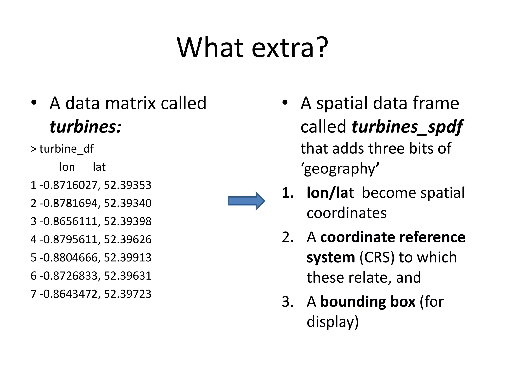
What extra? • A data matrix called • A spatial data frame turbines: called turbines_spdf > turbine_df that adds three bits of lon lat ‘geography’ 1 -0.8716027, 52.39353 1. lon/lat become spatial 2 -0.8781694, 52.39340 3 -0.8656111, 52.39398 coordinates 4 -0.8795611, 52.39626 2. A coordinate reference 5 -0.8804666, 52.39913 system (CRS) to which 6 -0.8726833, 52.39631 these relate, and 7 -0.8643472, 52.39723 3. A bounding box (for display)

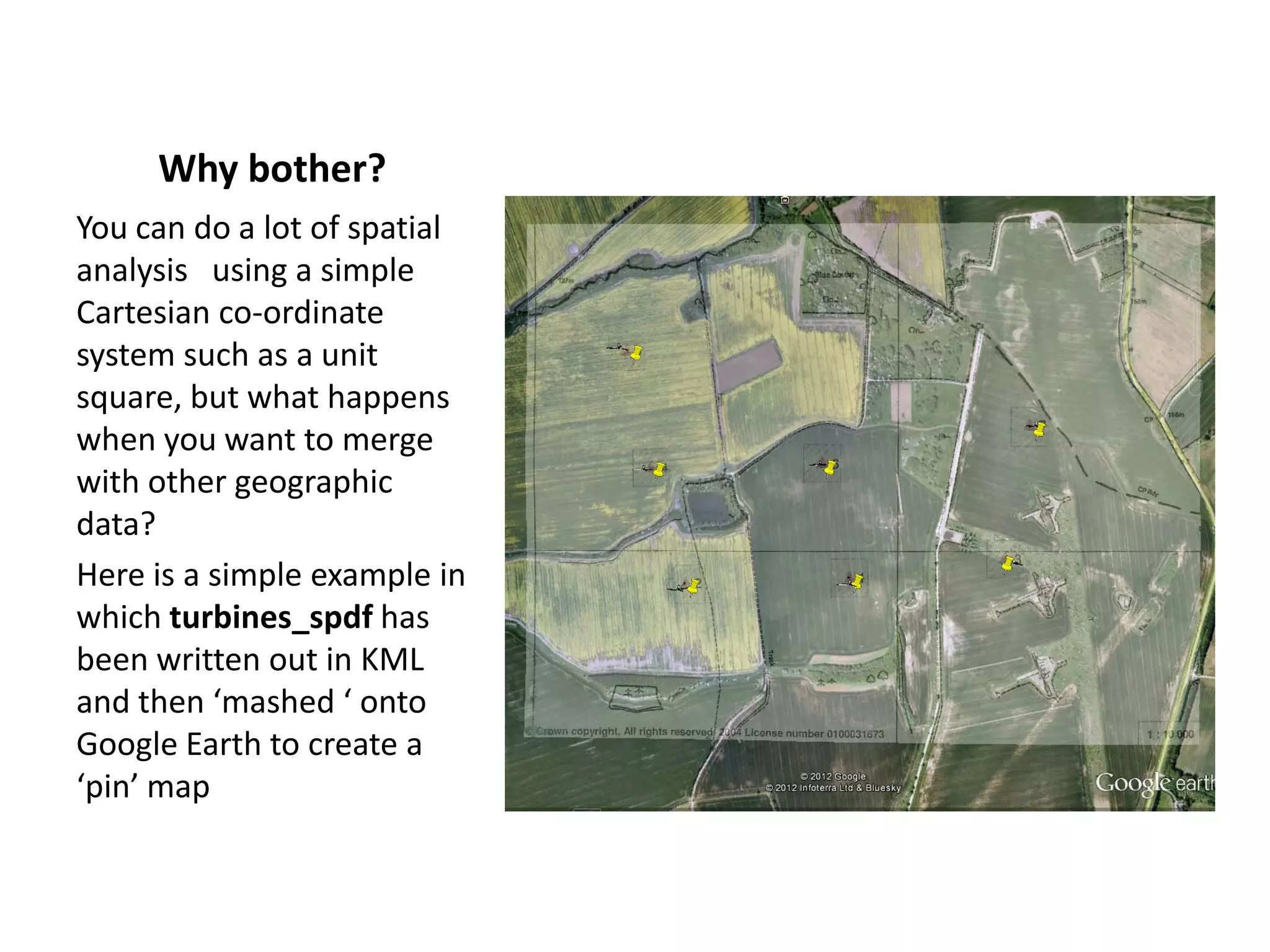
Why bother? You can do a lot of spatial analysis using a simple Cartesian co-ordinate system such as a unit square, but what happens when you want to merge with other geographic data? Here is a simple example in which turbines_spdf has been written out in KML and then ‘mashed ‘ onto Google Earth to create a ‘pin’ map

Packages for spatial data Contributed packages with spatial statistics applications: • Utilities: rgdal, sp, maptools • Point patterns: spatstat, VR:spatial, splancs; • Geostatistics: gstat, geoR, geoRglm, fields, spBayes, • RandomFields, VR: spatial, sgeostat, vardiag; • Lattice/area data: spdep, DCluster, spgwr, ade4.

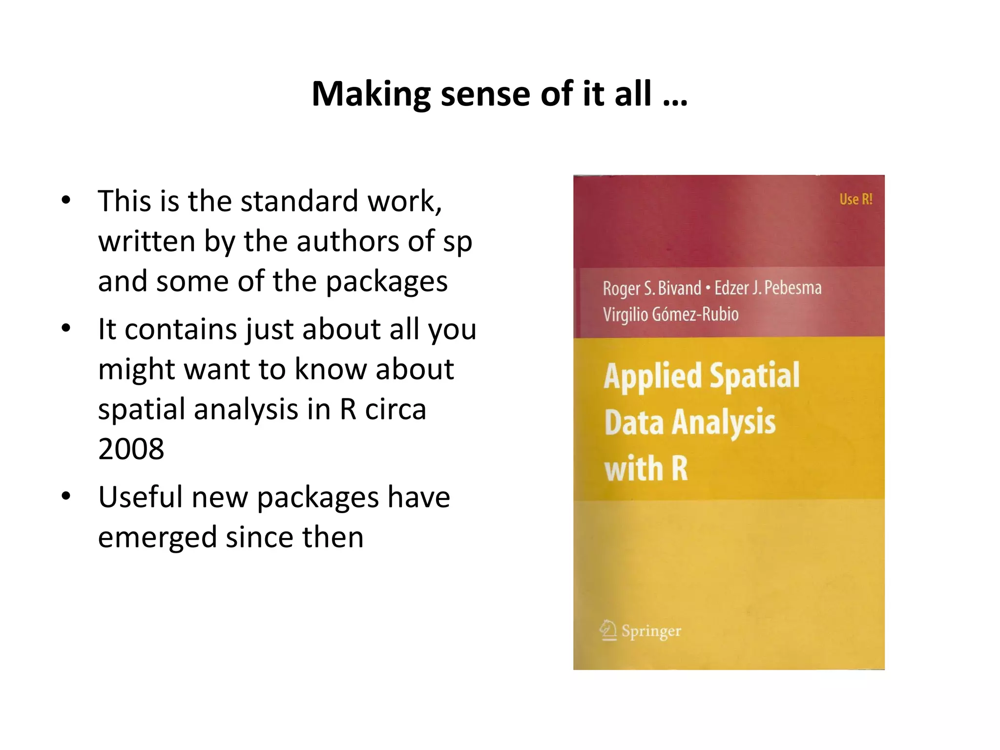
Making sense of it all … • This is the standard work, written by the authors of sp and some of the packages • It contains just about all you might want to know about spatial analysis in R circa 2008 • Useful new packages have emerged since then

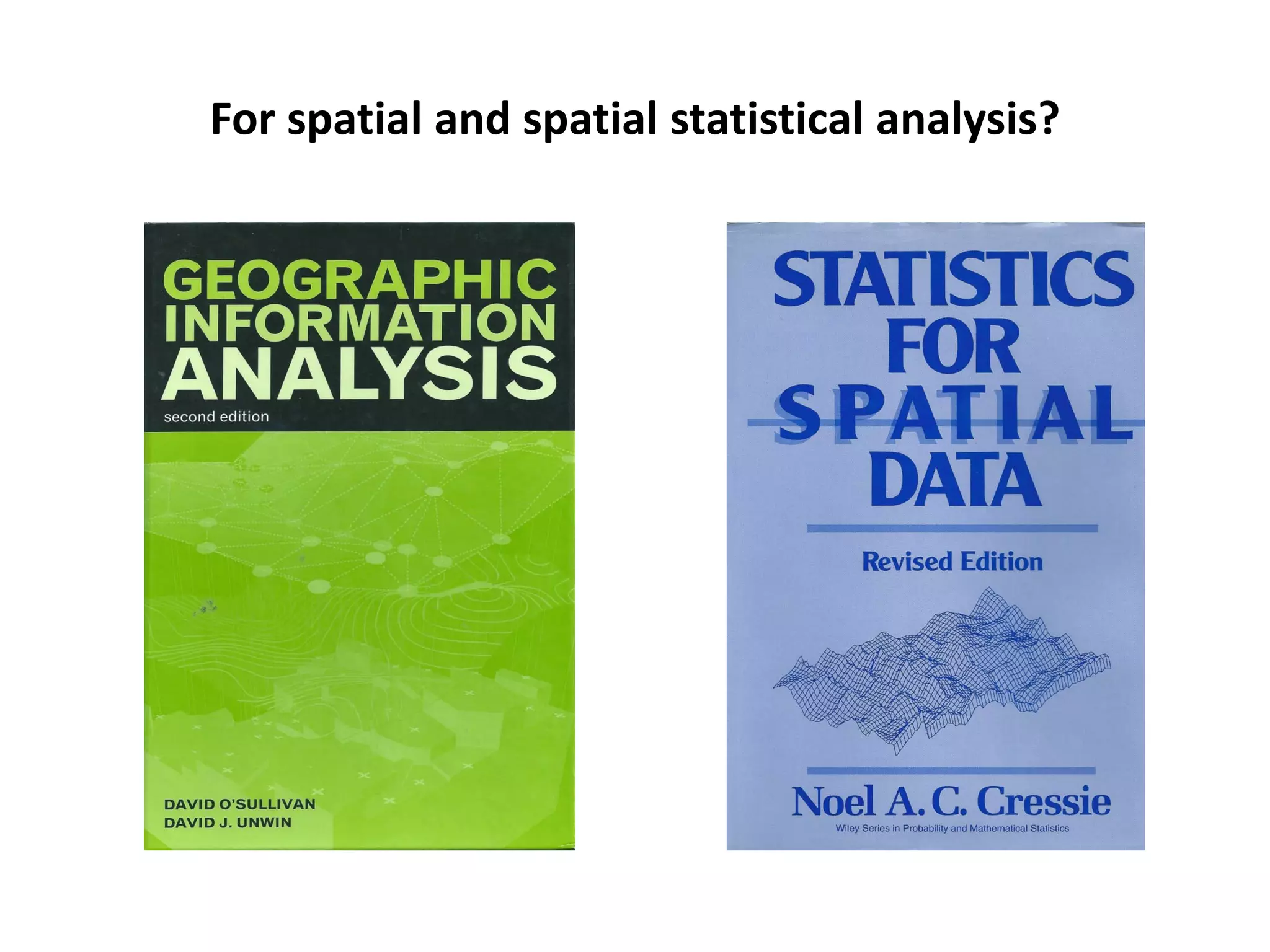
For spatial and spatial statistical analysis?

Three use case examples • Each illustrates the analysis of a particular class of spatial data -- points L0, area L2 and surfaces L3

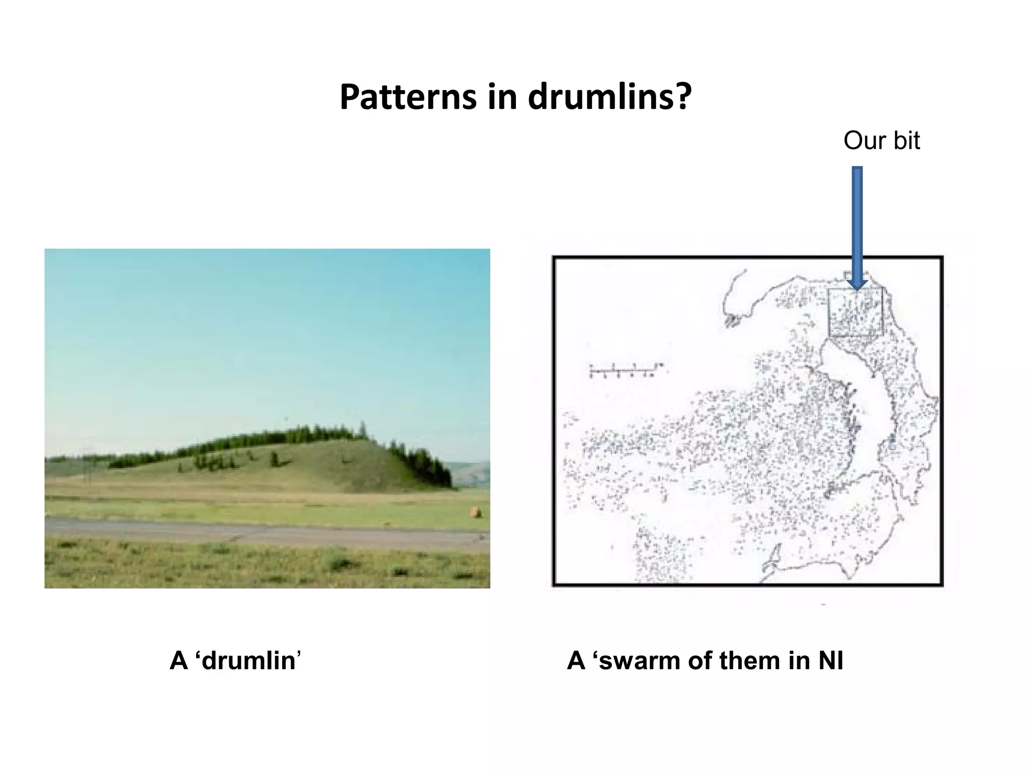
Patterns in drumlins? Our bit A ‘drumlin’ A ‘swarm of them in NI

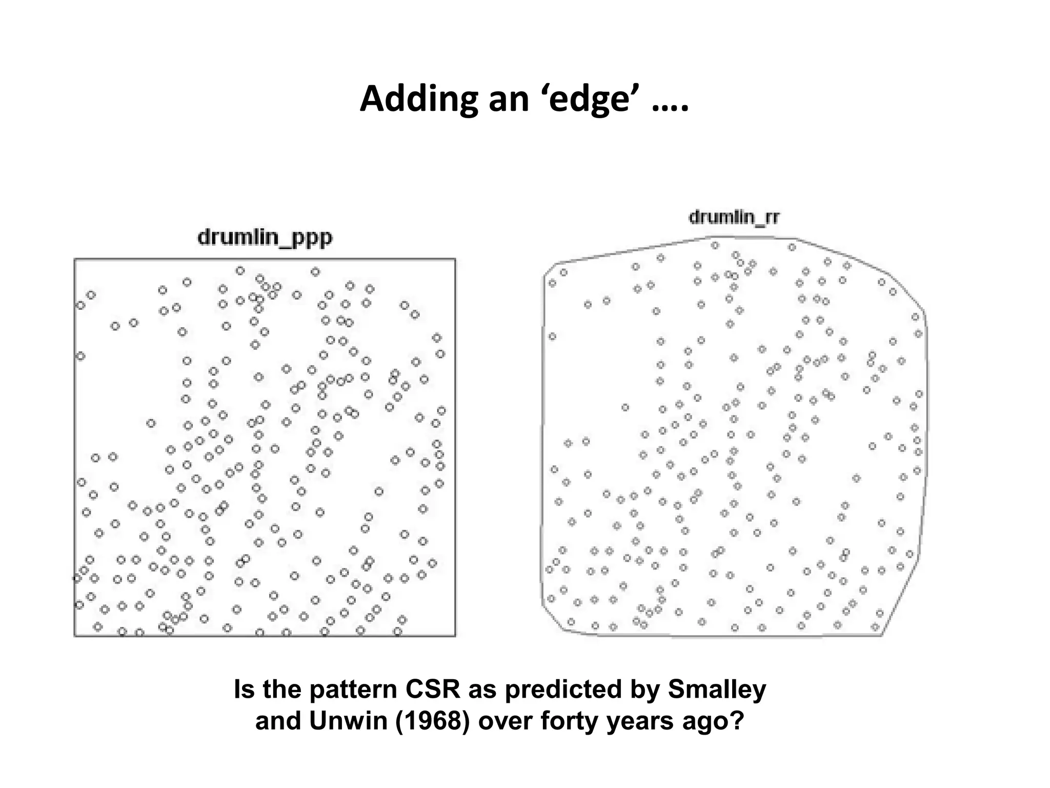
Adding an ‘edge’ …. Is the pattern CSR as predicted by Smalley and Unwin (1968) over forty years ago?

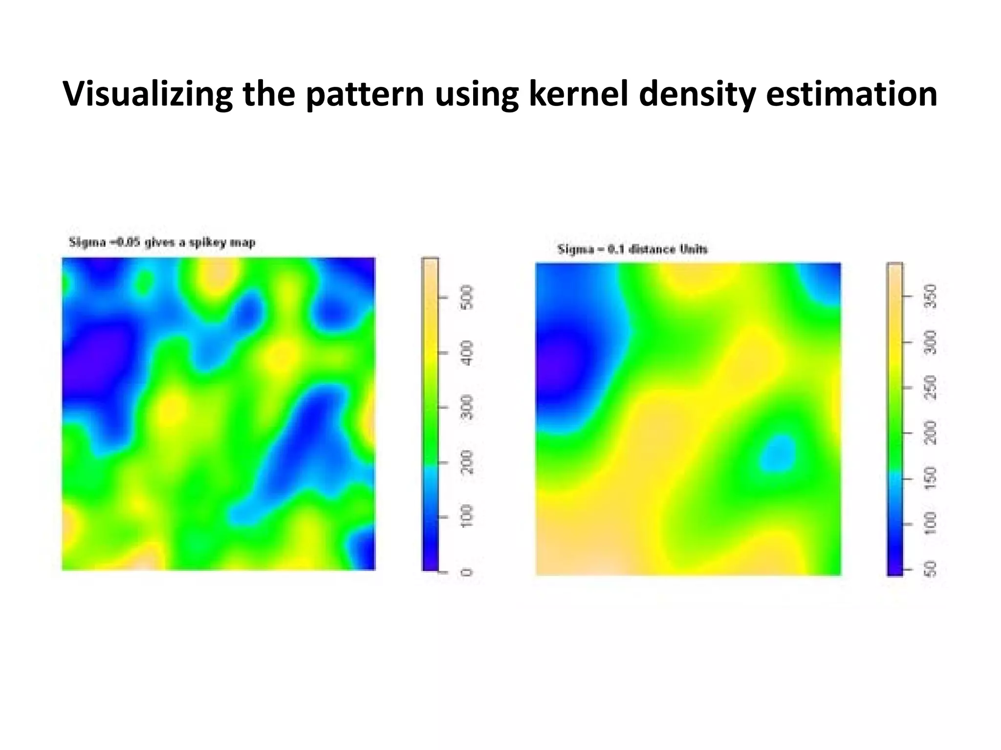
Visualizing the pattern using kernel density estimation

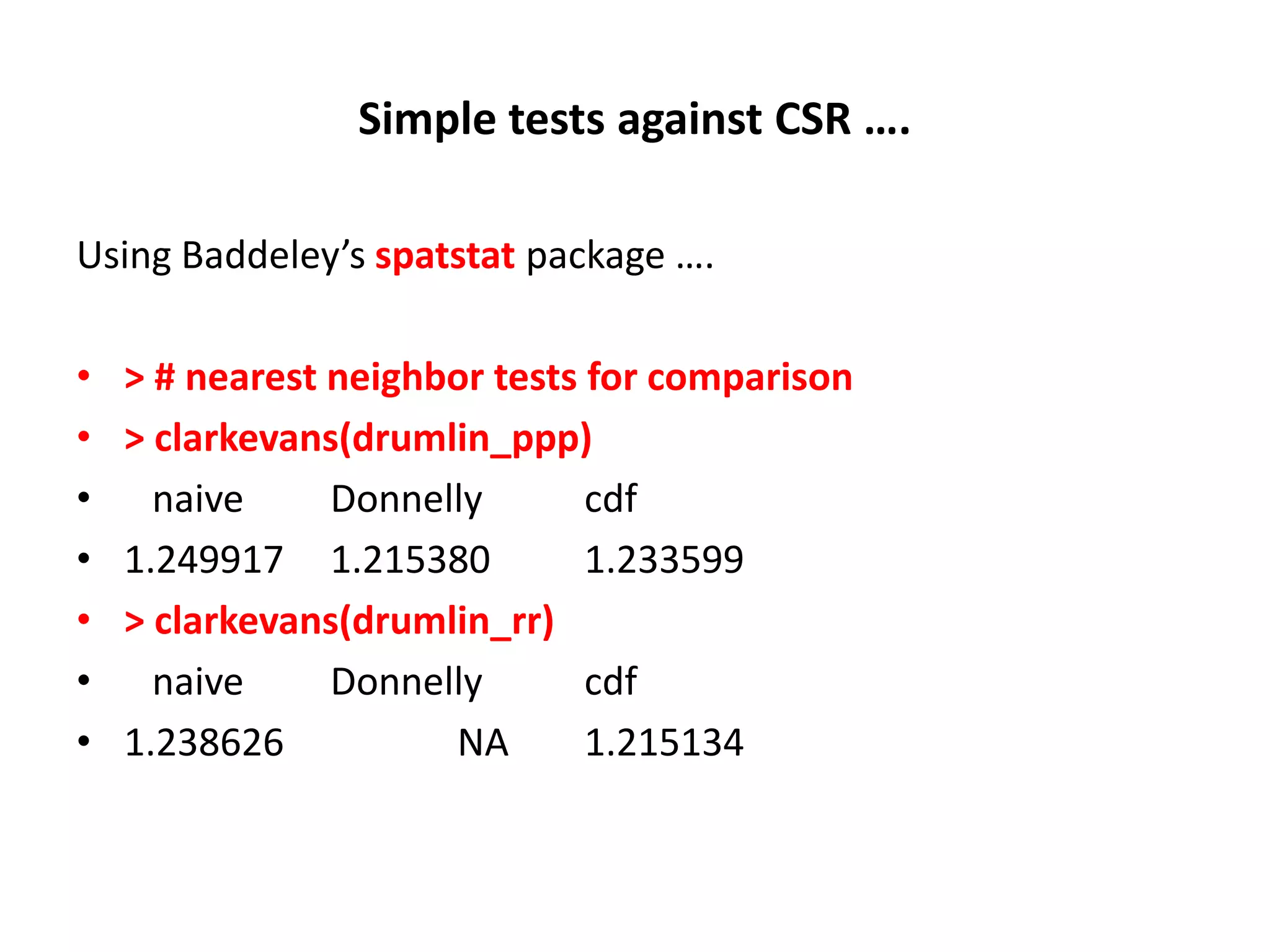
Simple tests against CSR …. Using Baddeley’s spatstat package …. • > # nearest neighbor tests for comparison • > clarkevans(drumlin_ppp) • naive Donnelly cdf • 1.249917 1.215380 1.233599 • > clarkevans(drumlin_rr) • naive Donnelly cdf • 1.238626 NA 1.215134

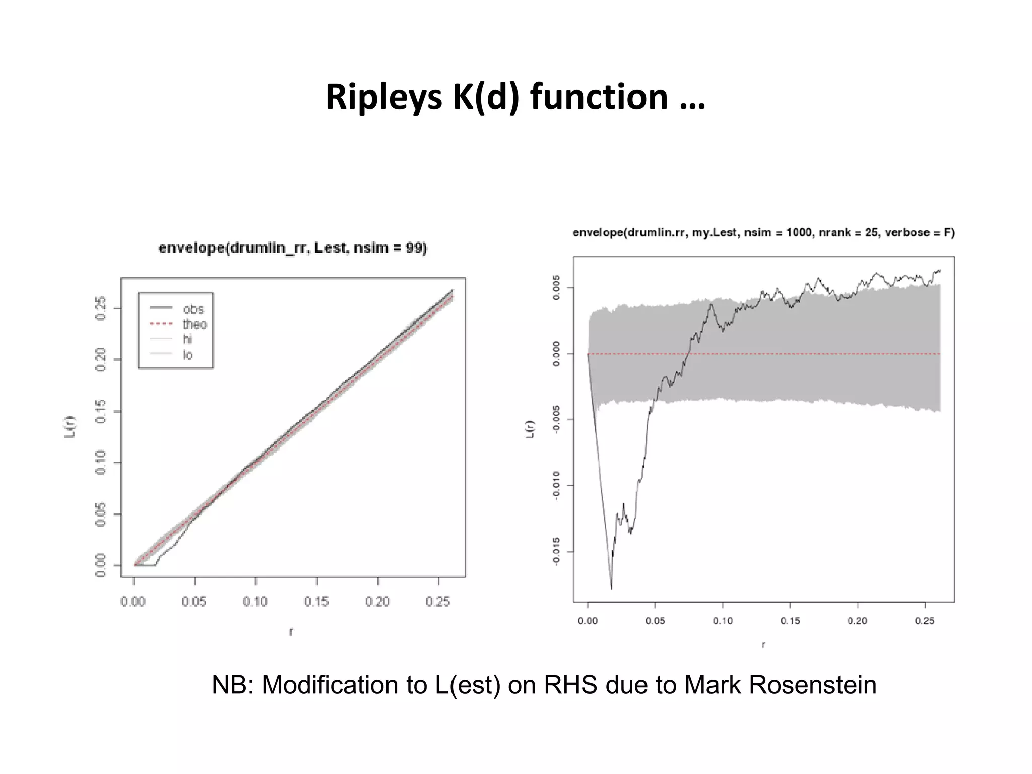
Ripleys K(d) function … NB: Modification to L(est) on RHS due to Mark Rosenstein

In this case we conclude that the pattern is more regular than random at short range, but then we have no evidence that it is other than CSR at longer ranges The generic question is Is there an unusual clustering of point objects such as crimes/cases of a disease/trees/ whatever here that we need to worry about? If so does the point pattern help explain why?

Patterns in disease incidence • Where does this disease occur? • Although disease affects individuals, almost always the available information will be aggregated into some areal unit such as a postal code, electoral district, county, state or country • Such data are called lattice data and they are visualized using choropleth (‘area-value’) maps • Our questions are essentially the same as before

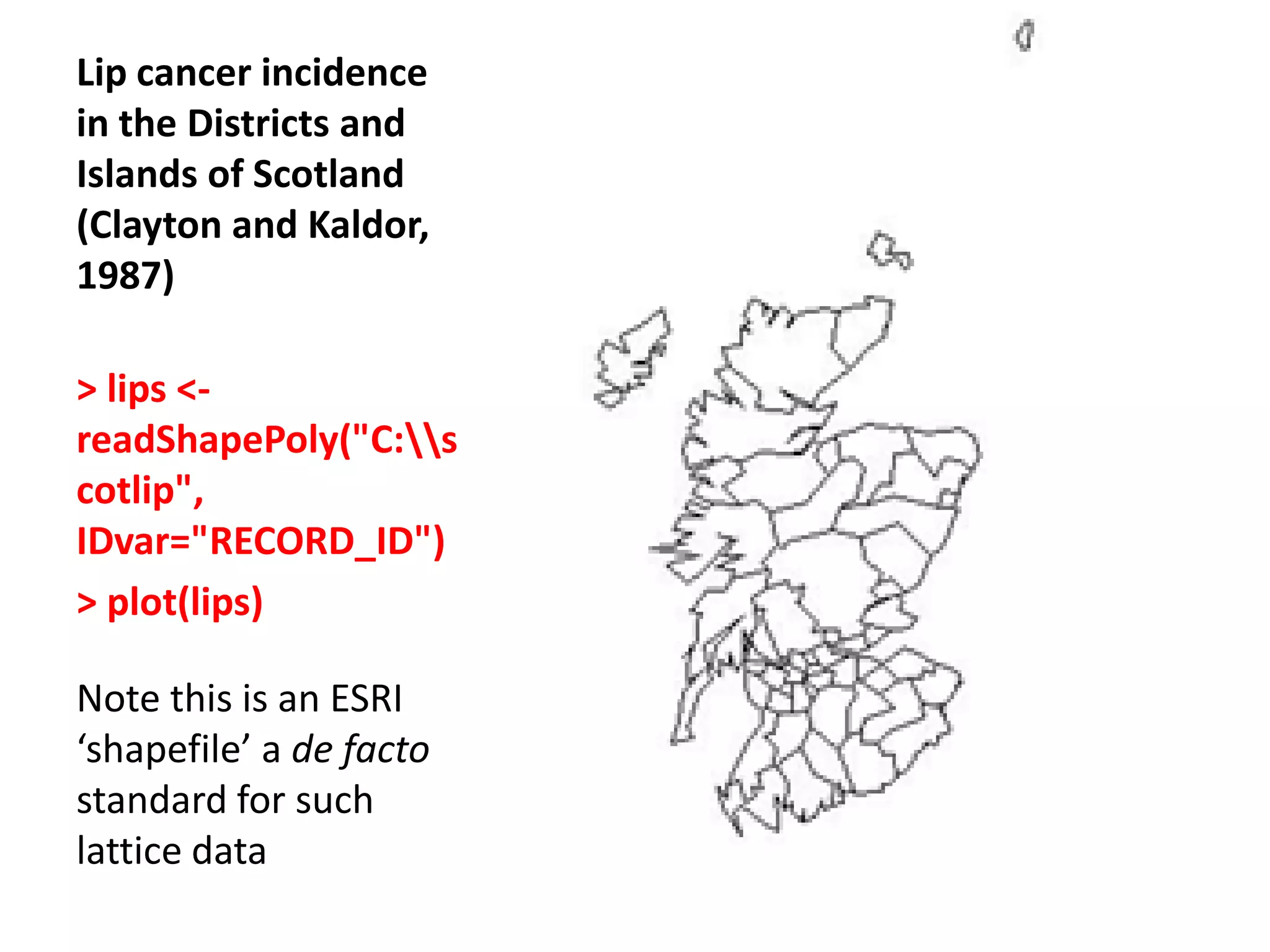
Lip cancer incidence in the Districts and Islands of Scotland (Clayton and Kaldor, 1987) > lips <- readShapePoly("C:s cotlip", IDvar="RECORD_ID") > plot(lips) Note this is an ESRI ‘shapefile’ a de facto standard for such lattice data

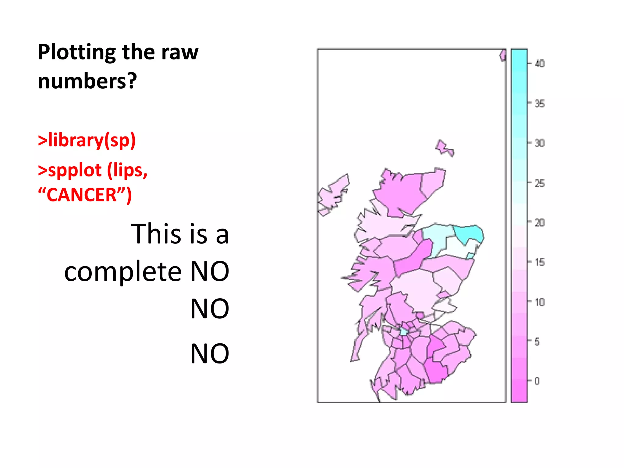
Plotting the raw numbers? >library(sp) >spplot (lips, “CANCER”) This is a complete NO NO NO

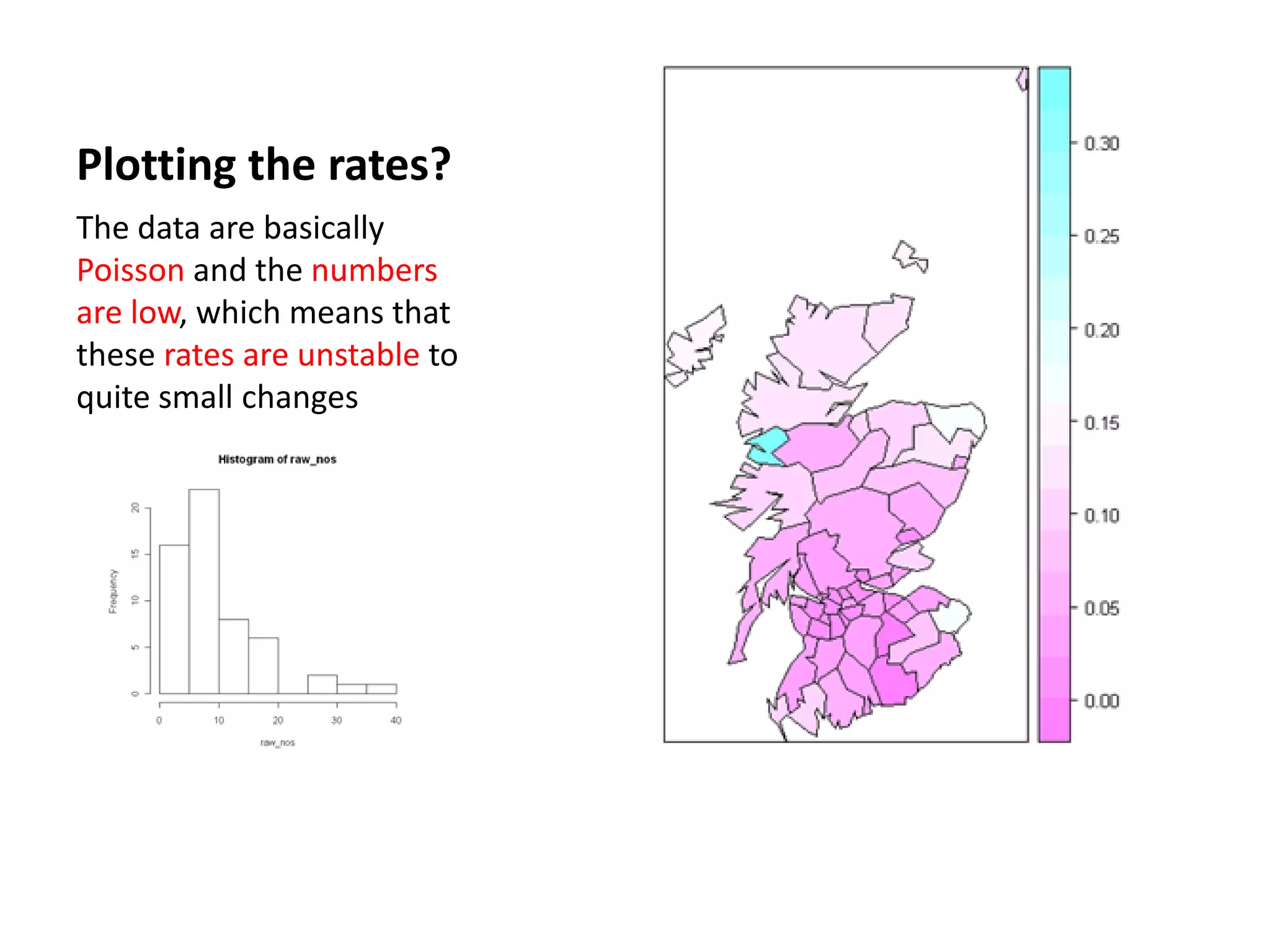
Plotting the rates? The data are basically Poisson and the numbers are low, which means that these rates are unstable to quite small changes

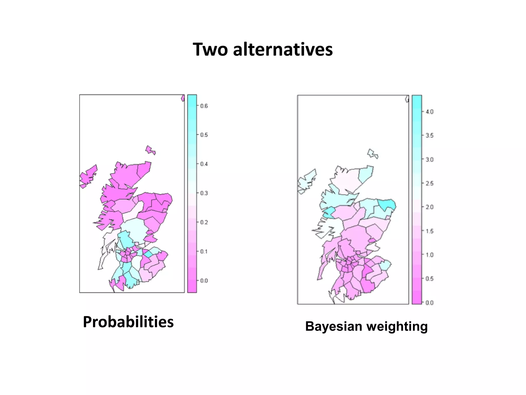
Two alternatives Probabilities Bayesian weighting

Chi-square mapping using ‘Pearsonian’ Residuals > sum(lips$CANCER) [1] 536 > sum(lips$POP) [1] 14979894 >pop_exp<- 536*(lips$POP/14979894) > chisq <- (lips$CANCER- pop_exp)/sqrt(pop_exp) > lips_chi <- spCbind(lips, chisq) >spplot(lips_chi,"chisq")

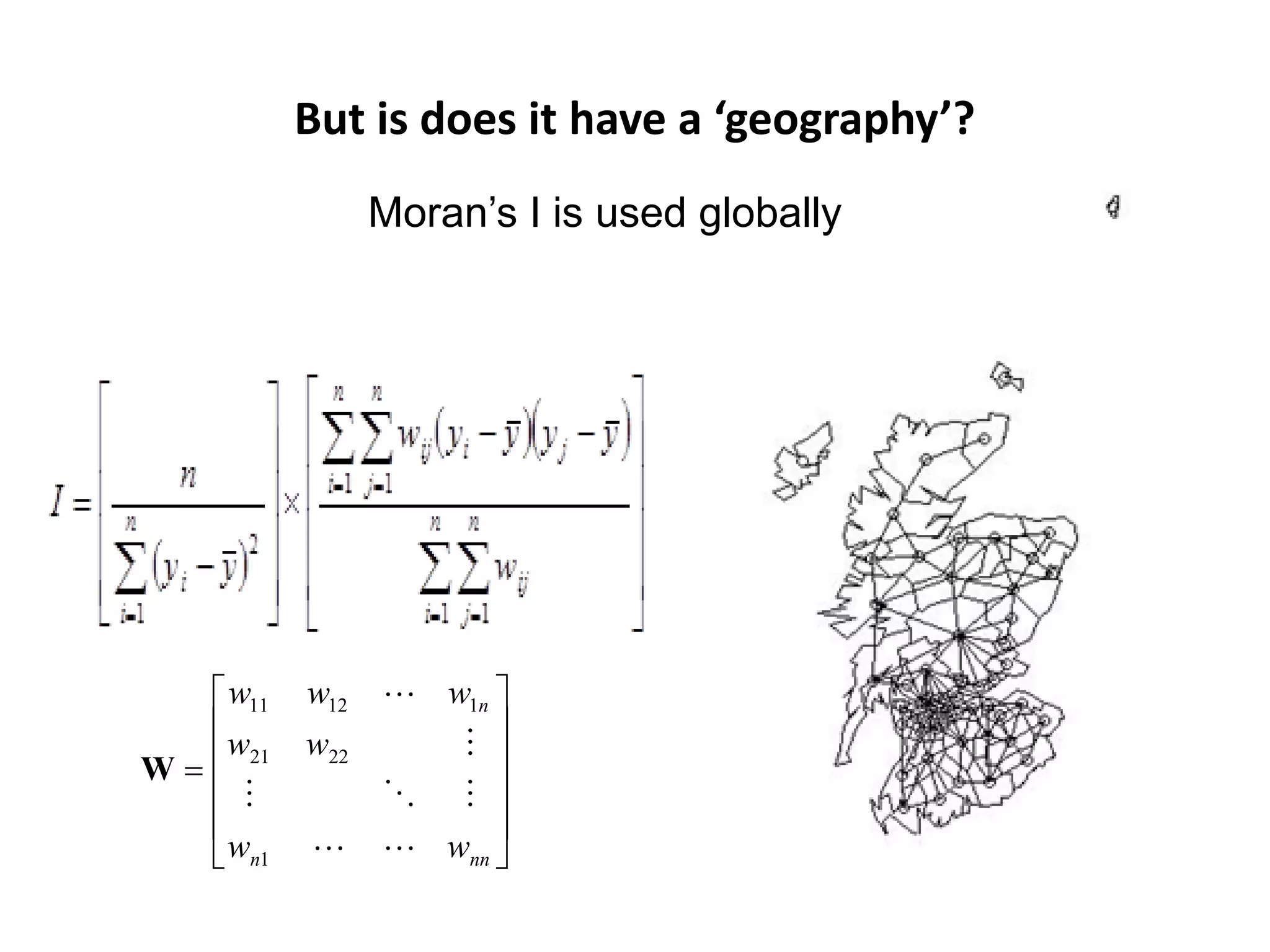
But is does it have a ‘geography’? Moran’s I is used globally  w11 w12  w1n  w w22   W =  21          wn1   wnn 

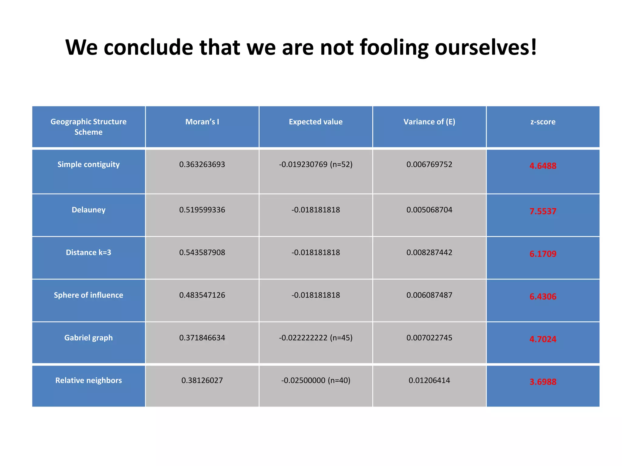
We conclude that we are not fooling ourselves! Geographic Structure Moran’s I Expected value Variance of (E) z-score Scheme Simple contiguity 0.363263693 -0.019230769 (n=52) 0.006769752 4.6488 Delauney 0.519599336 -0.018181818 0.005068704 7.5537 Distance k=3 0.543587908 -0.018181818 0.008287442 6.1709 Sphere of influence 0.483547126 -0.018181818 0.006087487 6.4306 Gabriel graph 0.371846634 -0.022222222 (n=45) 0.007022745 4.7024 Relative neighbors 0.38126027 -0.02500000 (n=40) 0.01206414 3.6988

We conclude that the pattern is ‘real’, the disease has a geography of interest The generic question is: Does this phenomenon in these areas (counties, states, countries) show spatial variation I need to know about? Does the pattern help explain why?

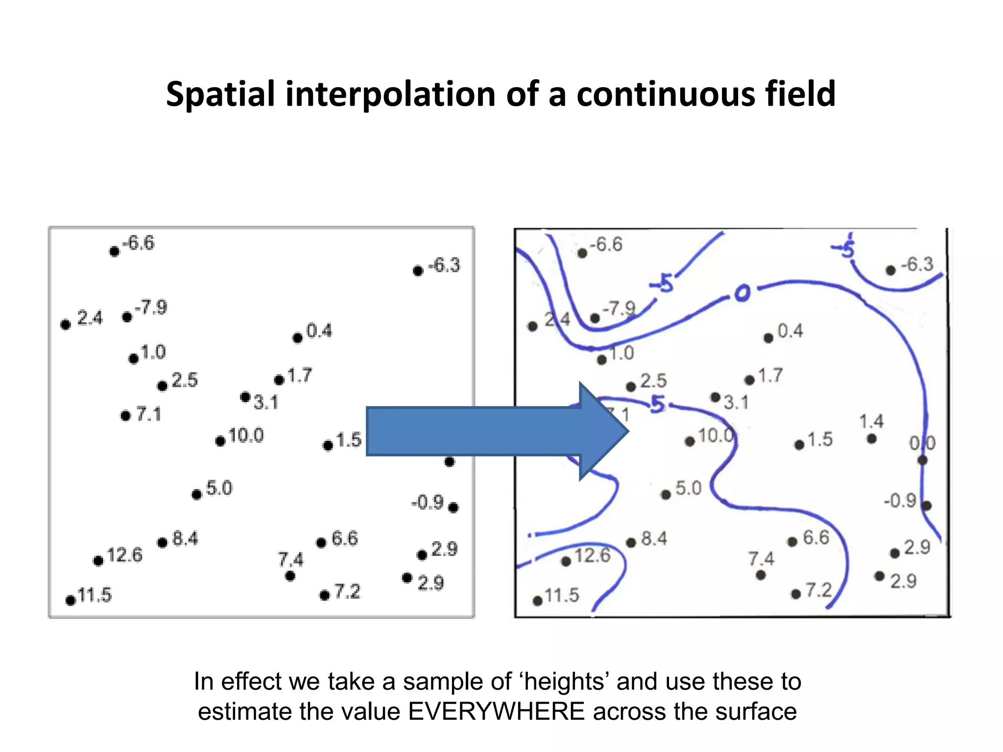
Spatial interpolation of a continuous field In effect we take a sample of ‘heights’ and use these to estimate the value EVERYWHERE across the surface

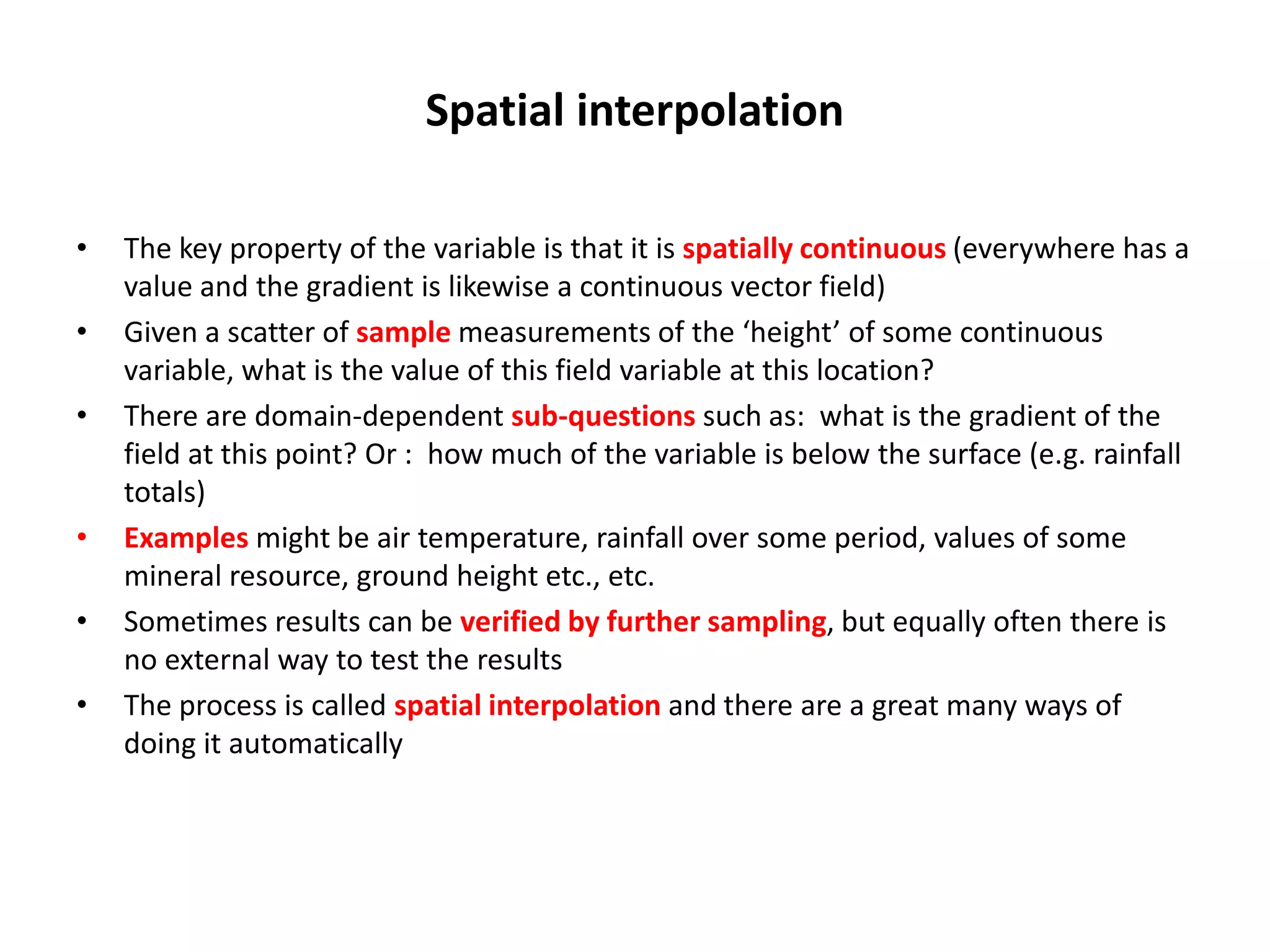
Spatial interpolation • The key property of the variable is that it is spatially continuous (everywhere has a value and the gradient is likewise a continuous vector field) • Given a scatter of sample measurements of the ‘height’ of some continuous variable, what is the value of this field variable at this location? • There are domain-dependent sub-questions such as: what is the gradient of the field at this point? Or : how much of the variable is below the surface (e.g. rainfall totals) • Examples might be air temperature, rainfall over some period, values of some mineral resource, ground height etc., etc. • Sometimes results can be verified by further sampling, but equally often there is no external way to test the results • The process is called spatial interpolation and there are a great many ways of doing it automatically

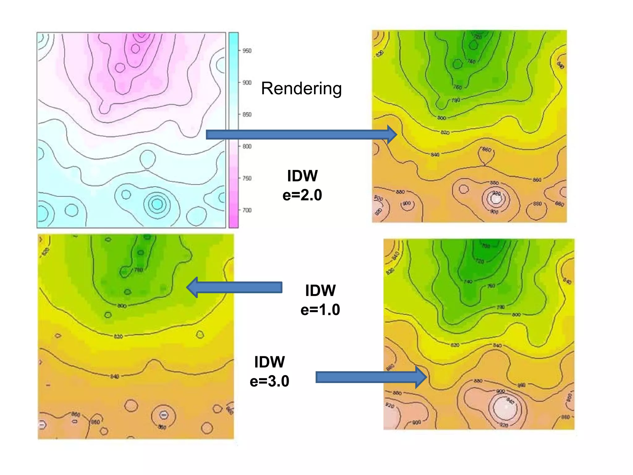
Interpolation by Inverse Distance Weighting (IDW) • Estimate each and every location on a very fine grid using an inverse distance weighted sum of the height values of neighboring control points • Uses the gstat package: • A parameter ‘e’ controls the degree of smoothing

Rendering IDW e=2.0 IDW e=1.0 IDW e=3.0

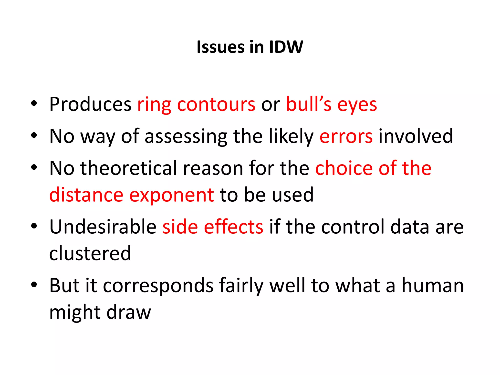
Issues in IDW • Produces ring contours or bull’s eyes • No way of assessing the likely errors involved • No theoretical reason for the choice of the distance exponent to be used • Undesirable side effects if the control data are clustered • But it corresponds fairly well to what a human might draw

Geostatistics: making use of spatial dependence in interpolation • For points and areas spatial dependence can complicate any statistical analysis using standard methods • Can we characterise the spatial dependence across a field and use it to produce better interpolations?

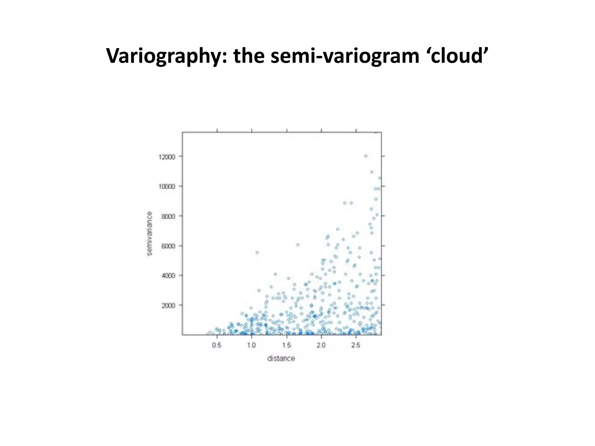
Variography: the semi-variogram ‘cloud’

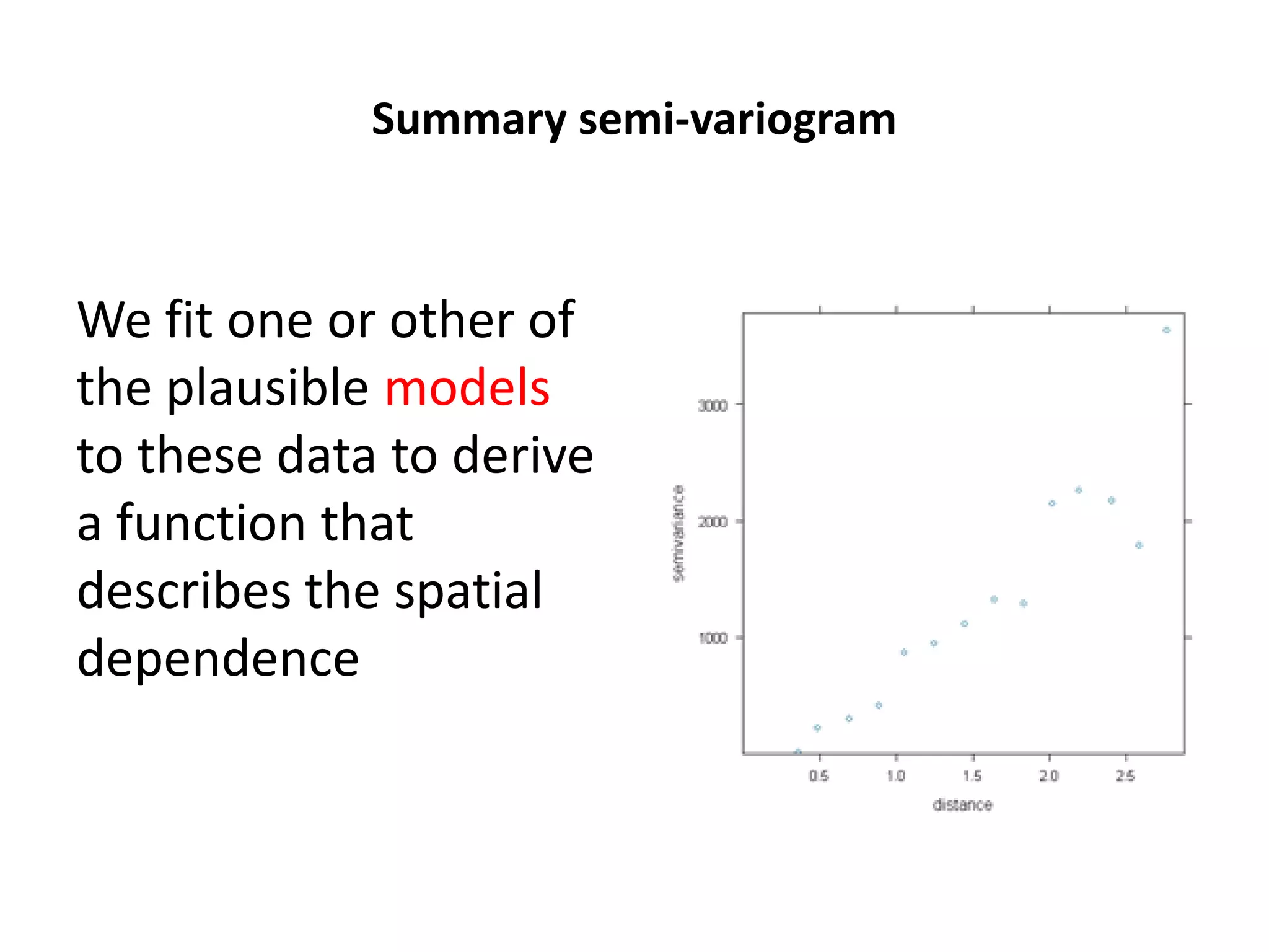
Summary semi-variogram We fit one or other of the plausible models to these data to derive a function that describes the spatial dependence

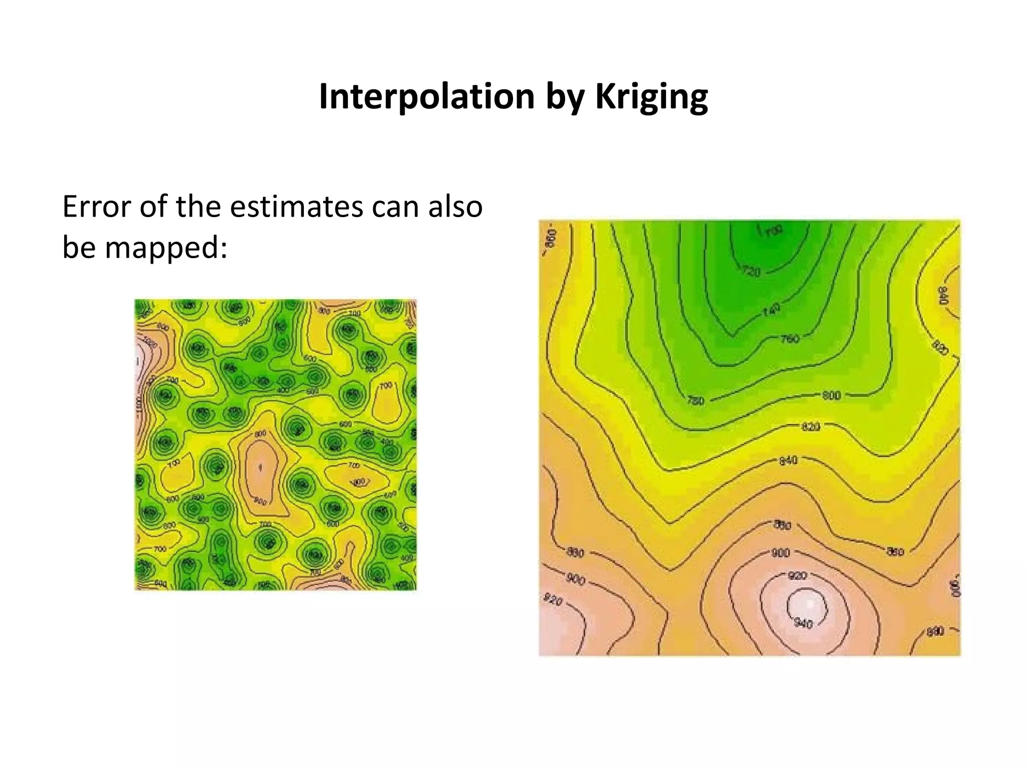
Interpolation by Kriging Error of the estimates can also be mapped:

We have our estimates over the entire area The generic question is: What is the most probable value for a continuous variable at this location?

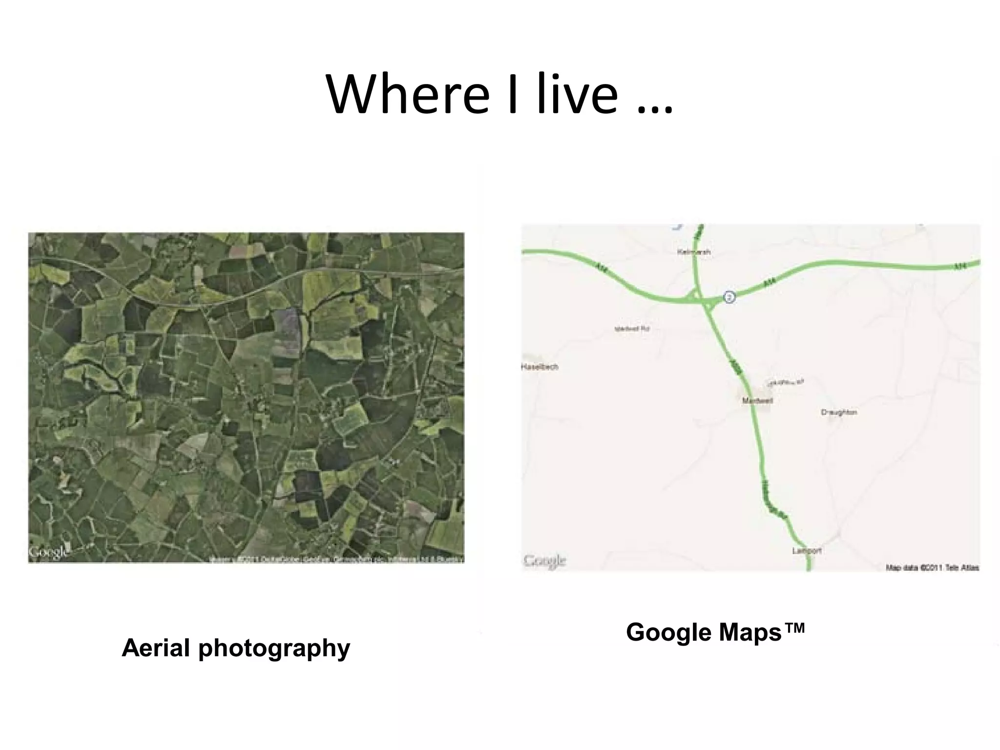
Some R-fun (1) : using dismo >library(XML) #needs this > library(rgdal) #and this >library (dismo) > place<-geocode("Maidwell, > size<-extent(unlist(place[4:7])) Northamptonshire, UK") #the #what does this do? address needs to have enough to be > map<-gmap(size,type="satellite") recognized > plot(map) > place # the place object is a vector > map<-gmap(size,type="roadmap") of length 7 with a bounding box: > plot(map) ID lon lat lonmin lonmax latmin latmax To find places and plot 1 1 -0.9030642 52.38524 -0.938073 them using Google -0.8710494 52.37016 52.40107 Earth and Maps™ location 1 Maidwell, Northamptonshire, UK

Where I live … Google Maps™ Aerial photography

Or (slightly) better known? > place<-geocode("The White House, Washington, USA") > size<- extent(unlist(place[4:7])) > map<- gmap(size,type="satellite") > plot(map)

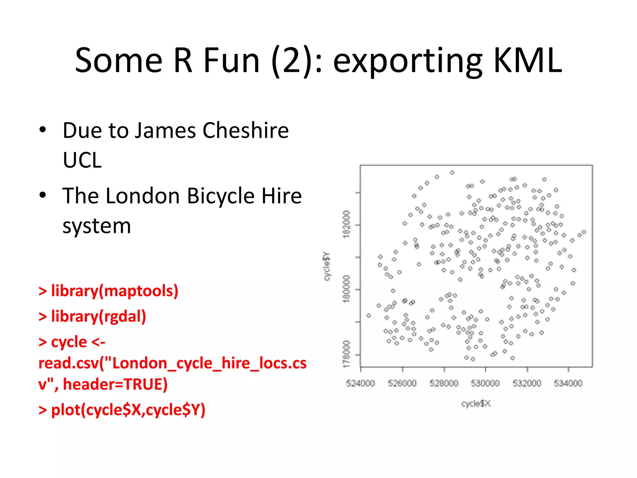
Some R Fun (2): exporting KML • Due to James Cheshire UCL • The London Bicycle Hire system > library(maptools) > library(rgdal) > cycle <- read.csv("London_cycle_hire_locs.cs v", header=TRUE) > plot(cycle$X,cycle$Y)

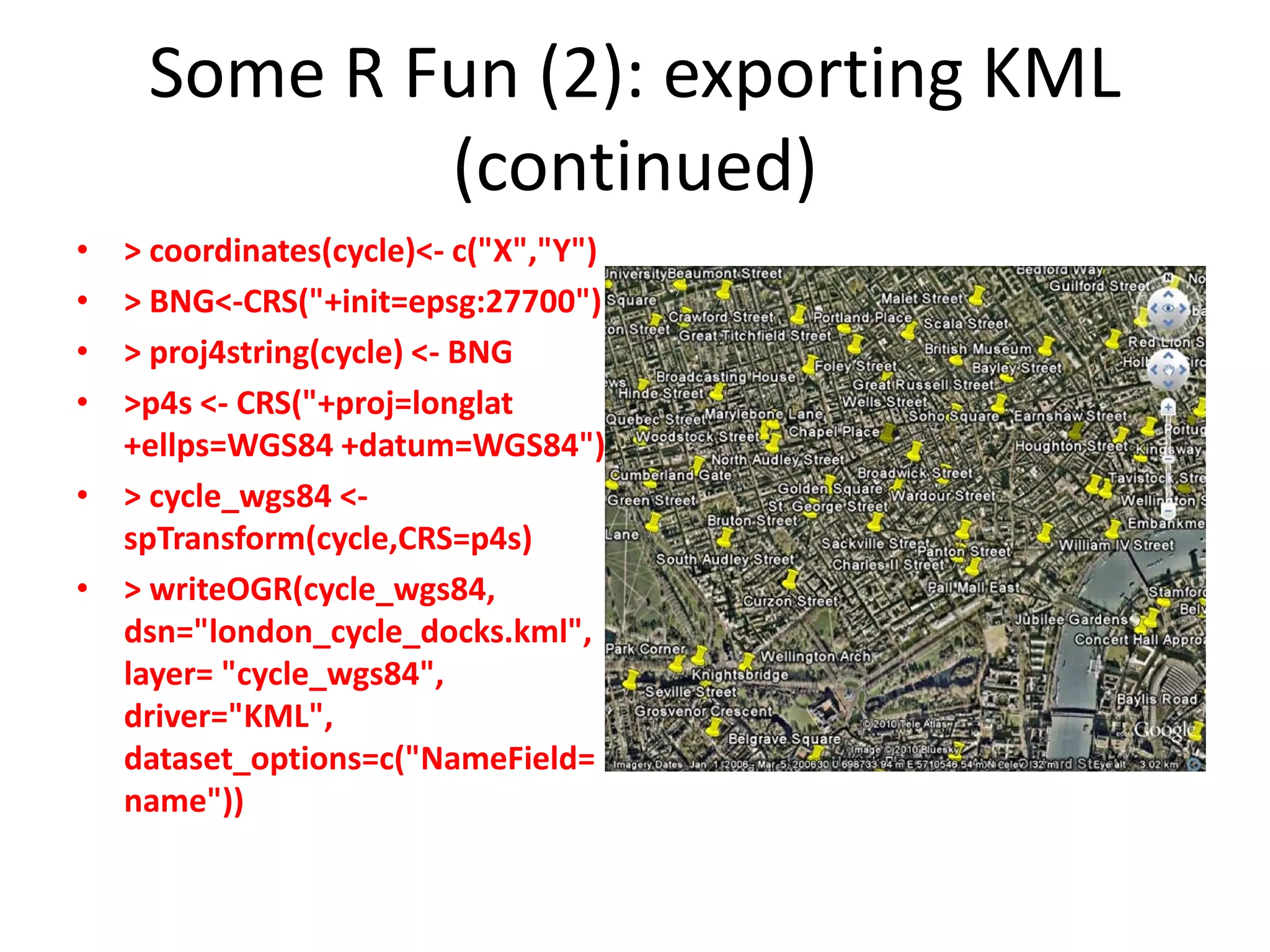
Some R Fun (2): exporting KML (continued) • > coordinates(cycle)<- c("X","Y") • > BNG<-CRS("+init=epsg:27700") • > proj4string(cycle) <- BNG • >p4s <- CRS("+proj=longlat +ellps=WGS84 +datum=WGS84") • > cycle_wgs84 <- spTransform(cycle,CRS=p4s) • > writeOGR(cycle_wgs84, dsn="london_cycle_docks.kml", layer= "cycle_wgs84", driver="KML", dataset_options=c("NameField= name"))

The End • Taking it further: • Applied Spatial Data Analysis with R (Bivand, Pebesma and Gomez-Rubio (2008) • Spatial Statistics with R commences 14th December 2012 at Statistics.com ™ QUESTIONS ARE WELCOME

Finding Meaning in Points, Areas and Surfaces: Spatial Analysis in R

More Related Content

What's hot

Viewers also liked

Similar to Finding Meaning in Points, Areas and Surfaces: Spatial Analysis in R

More from Revolution Analytics

Recently uploaded

Finding Meaning in Points, Areas and Surfaces: Spatial Analysis in R