Generating test data for Statistical and ML models

TEST DATA FOR ML … or what’s for your models fit() ...

Preface When you are working with Machine Learning, Neural Networks, and similar technologies, one problem that you will need to solve, is test datasets. There are many datasets already exists. “All time classic” Iris dataset. Or character recognition dataset. Or house prices datasets. New datasets appearing almost daily on Kaggle. And this is good. But we always wants more. The new dataset that we can crave, are usually the “windows to an uncharted territories”, which we can somehow define, but the data that we receiving are inconclusive ? Or we are training our Neural Net to search for the patterns in our input data, so somehow we shall provide it a patterns ? Or shall we create such patterns artificially, to help with a proper recognition ? All those cases, and more are calling for controllable generation of the input data for the Machine Learning. And “Jmaster” is an answer to that call.

About me My name is Vladimir Ulogov, and I’ve been around for a while. I’ve been a Systems Engineer, Administrator, Software Developer, Monitoring expert for almost 30 years. Worked with Statistical data and models for a decades and developed a number of internal tools, that’s I’ve used to test those models. You probably says: “Why the heck, the Systems Engineer needs statistics ?”. The answer will be: “For a lot and lot of reasons”. Statistical computations is a cornerstone for a metrics computations and monitoring. They are invaluable in performance monitoring and capacity planning. You can not do any kind of analytics without them. Security monitoring, analysis of the pen-testing and traffic analysis ? Don’t even think about it if you are not good with Statistical computations. And in recent years, new and useful development emerged - Machine Learning. While it is not directly related to a Statistics, ML methods and techniques compliments and surpassing some of the “good ol’ tried and true” methods, and they quickly become a cornerstone for a large number of the instruments, used by Systems Engineers around the world. And while I am joining the ranks of the engineers who is designing and developing “the tools of the trade”, I am developing some tools for myself.

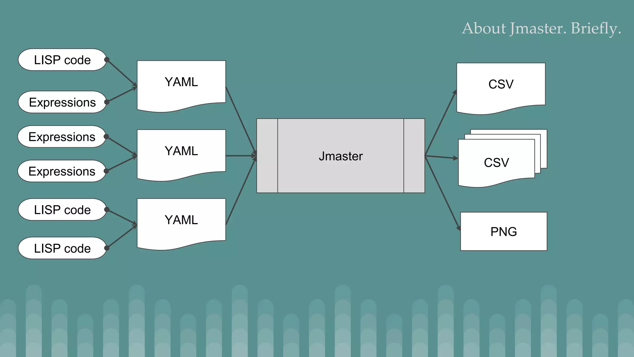
About Jmaster. Briefly. Jmaster is an instrument, for generating user-controlled and user-defined datasets, that could be used for testing ether Statistical or ML models. How this works ? To test Statistical or ML models, we do need to feed them with controllable data, that will help us to assess how the behaviour of the model matches our expectation. This data is produced in the form of CSV files and some PNG files, which helping us to estimate the quality of the generated data. As an input for this tool, we are using YAML file in which we describing “the model”. This “model” is definition of how our data is generated. In addition to the data, Jmaster generating some images, helping us to assess the quality of generated data. So, some YAML on input and CSV and PNG files on output. Data, that is stored in CSV files, actually is columnar storage, where every column is a specific attribute. Developer of YAML models defining the size of the attribute, or “number of rows”. In this version of the tool, all generations are finite. I.e. “streaming mode” is not available. In current version, there are two modes for generation logic. A “model” mode and “time series mode”. I will explain of what they are shortly.

About Jmaster. Briefly. Jmaster YAML YAML YAML LISP code Expressions Expressions Expressions LISP code LISP code CSV CSV PNG

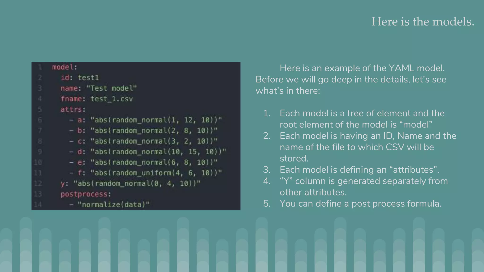
Here is the models. Here is an example of the YAML model. Before we will go deep in the details, let’s see what’s in there: 1. Each model is a tree of element and the root element of the model is “model” 2. Each model is having an ID, Name and the name of the file to which CSV will be stored. 3. Each model is defining an “attributes”. 4. “Y” column is generated separately from other attributes. 5. You can define a post process formula.

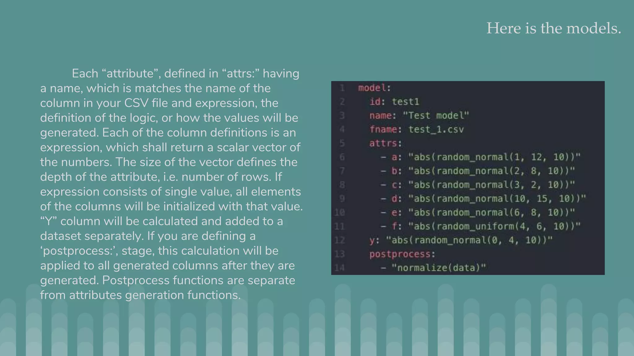
Here is the models. Each “attribute”, defined in “attrs:” having a name, which is matches the name of the column in your CSV file and expression, the definition of the logic, or how the values will be generated. Each of the column definitions is an expression, which shall return a scalar vector of the numbers. The size of the vector defines the depth of the attribute, i.e. number of rows. If expression consists of single value, all elements of the columns will be initialized with that value. “Y” column will be calculated and added to a dataset separately. If you are defining a ‘postprocess:’, stage, this calculation will be applied to all generated columns after they are generated. Postprocess functions are separate from attributes generation functions.

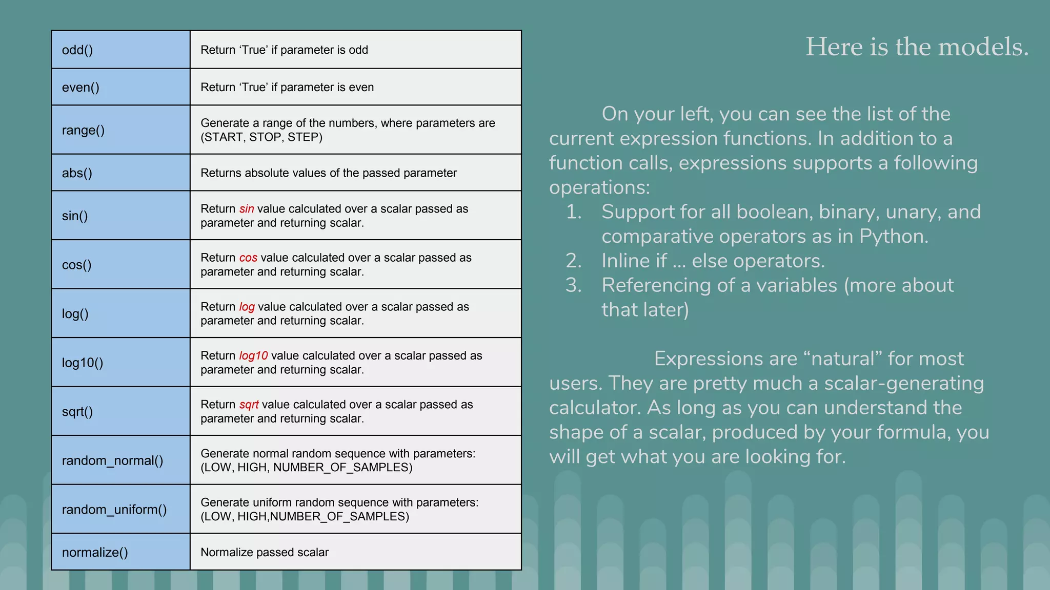
Here is the models. On your left, you can see the list of the current expression functions. In addition to a function calls, expressions supports a following operations: 1. Support for all boolean, binary, unary, and comparative operators as in Python. 2. Inline if … else operators. 3. Referencing of a variables (more about that later) Expressions are “natural” for most users. They are pretty much a scalar-generating calculator. As long as you can understand the shape of a scalar, produced by your formula, you will get what you are looking for. odd() Return ‘True’ if parameter is odd even() Return ‘True’ if parameter is even range() Generate a range of the numbers, where parameters are (START, STOP, STEP) abs() Returns absolute values of the passed parameter sin() Return sin value calculated over a scalar passed as parameter and returning scalar. cos() Return cos value calculated over a scalar passed as parameter and returning scalar. log() Return log value calculated over a scalar passed as parameter and returning scalar. log10() Return log10 value calculated over a scalar passed as parameter and returning scalar. sqrt() Return sqrt value calculated over a scalar passed as parameter and returning scalar. random_normal() Generate normal random sequence with parameters: (LOW, HIGH, NUMBER_OF_SAMPLES) random_uniform() Generate uniform random sequence with parameters: (LOW, HIGH,NUMBER_OF_SAMPLES) normalize() Normalize passed scalar

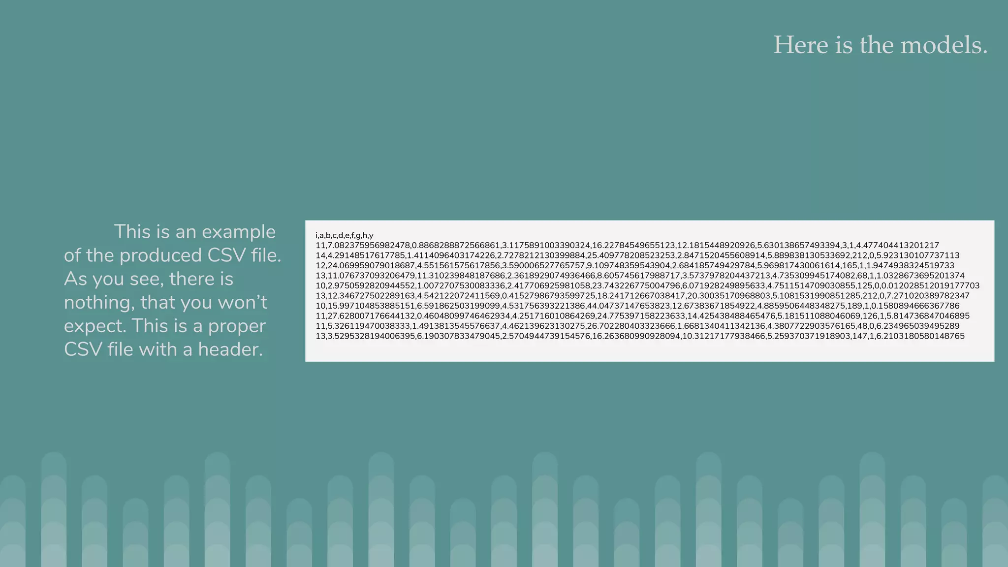
Here is the models. This is an example of the produced CSV file. As you see, there is nothing, that you won’t expect. This is a proper CSV file with a header. i,a,b,c,d,e,f,g,h,y 11,7.082375956982478,0.8868288872566861,3.1175891003390324,16.22784549655123,12.1815448920926,5.630138657493394,3,1,4.477404413201217 14,4.29148517617785,1.4114096403174226,2.7278212130399884,25.409778208523253,2.8471520455608914,5.889838130533692,212,0,5.923130107737113 12,24.069959079018687,4.551561575617856,3.590006527765757,9.109748359543904,2.684185749429784,5.969817430061614,165,1,1.9474938324519733 13,11.076737093206479,11.310239848187686,2.3618929074936466,8.605745617988717,3.5737978204437213,4.735309945174082,68,1,1.0328673695201374 10,2.9750592820944552,1.0072707530083336,2.417706925981058,23.743226775004796,6.071928249895633,4.7511514709030855,125,0,0.012028512019177703 13,12.346727502289163,4.542122072411569,0.41527986793599725,18.241712667038417,20.30035170968803,5.1081531990851285,212,0,7.271020389782347 10,15.997104853885151,6.591862503199099,4.531756393221386,44.04737147653823,12.67383671854922,4.8859506448348275,189,1,0.1580894666367786 11,27.628007176644132,0.46048099746462934,4.251716010864269,24.775397158223633,14.425438488465476,5.181511088046069,126,1,5.814736847046895 11,5.326119470038333,1.4913813545576637,4.462139623130275,26.702280403323666,1.6681340411342136,4.3807722903576165,48,0,6.234965039495289 13,3.5295328194006395,6.190307833479045,2.5704944739154576,16.263680990928094,10.31217177938466,5.259370371918903,147,1,6.2103180580148765

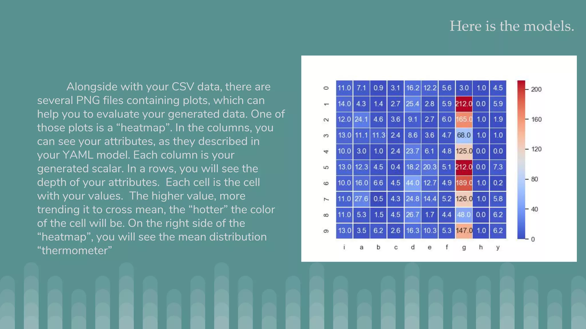
Here is the models. Alongside with your CSV data, there are several PNG files containing plots, which can help you to evaluate your generated data. One of those plots is a “heatmap”. In the columns, you can see your attributes, as they described in your YAML model. Each column is your generated scalar. In a rows, you will see the depth of your attributes. Each cell is the cell with your values. The higher value, more trending it to cross mean, the “hotter” the color of the cell will be. On the right side of the “heatmap”, you will see the mean distribution “thermometer”

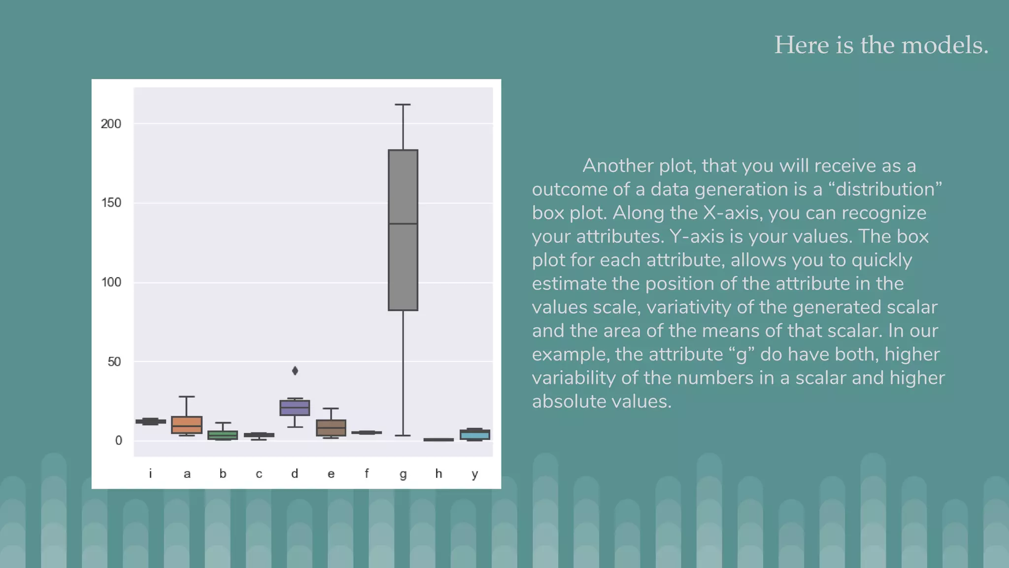
Here is the models. Another plot, that you will receive as a outcome of a data generation is a “distribution” box plot. Along the X-axis, you can recognize your attributes. Y-axis is your values. The box plot for each attribute, allows you to quickly estimate the position of the attribute in the values scale, variativity of the generated scalar and the area of the means of that scalar. In our example, the attribute “g” do have both, higher variability of the numbers in a scalar and higher absolute values.

Here is the models. I’ve already mentioned, that the expressions can reference a variables. And now it is time to show how to define and use them. There are element in the YAML file called “variables:” and elements referred by that element are variables definitions. Where element “name” is a variable name and element “value” is an expression, which will be evaluated and result of evaluation will be assigned to that variable. Please note, once variable defined, it’s become to known to all subsequently performed evaluations. This means, that for Jmaster all variables are global. I’ve decided not to go with complexities of the context’s for such simple tool. Here is where you will define a variables. Please also note: The variable names and attribute names are not mixing in the same context. I am deliberately defined variable “a” and assigned to it a scalar of 10 integers randomly generated with low-mark 0 and high- mark 255, and attribute “a”, which is calling function normalize() and referring a variable “a” as parameter for that function.

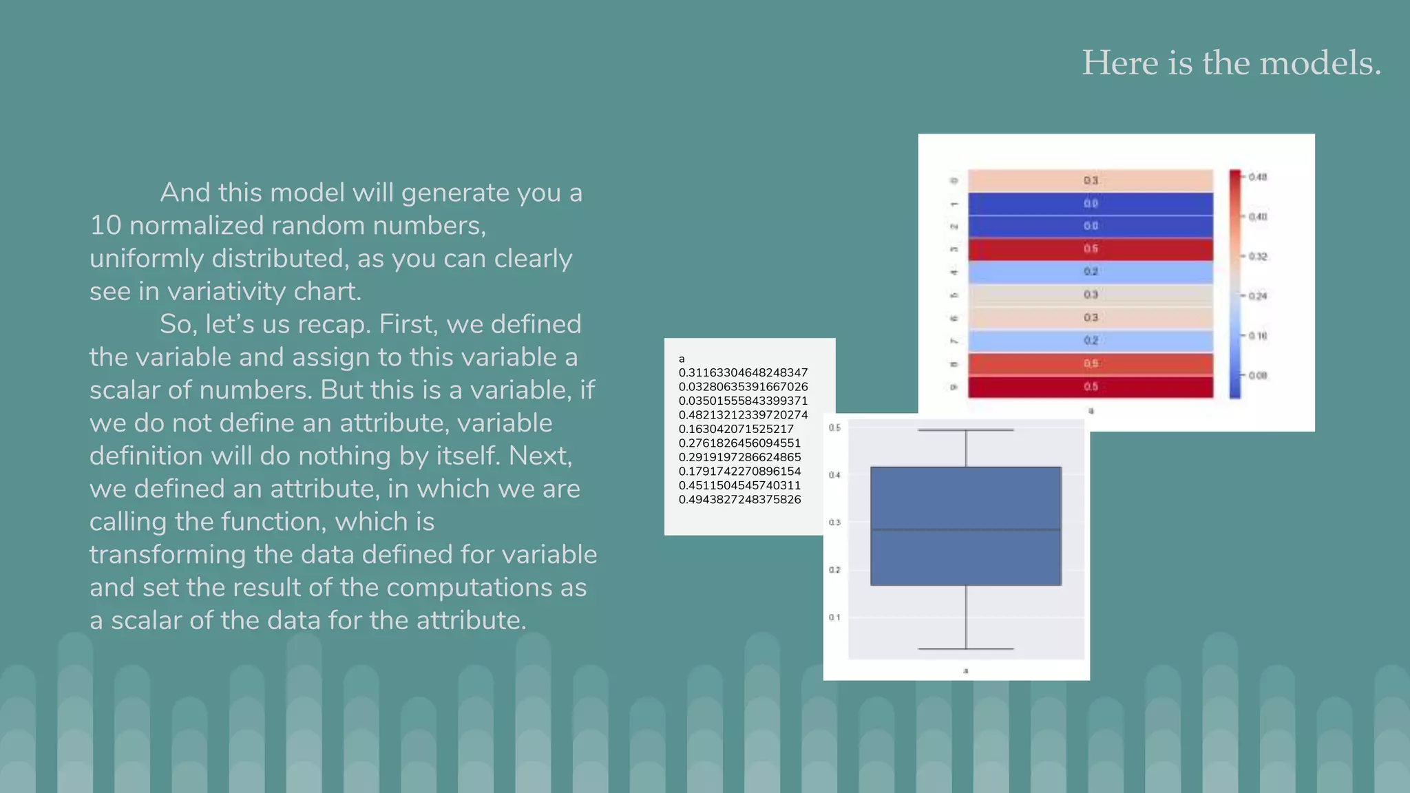
Here is the models. And this model will generate you a 10 normalized random numbers, uniformly distributed, as you can clearly see in variativity chart. So, let’s us recap. First, we defined the variable and assign to this variable a scalar of numbers. But this is a variable, if we do not define an attribute, variable definition will do nothing by itself. Next, we defined an attribute, in which we are calling the function, which is transforming the data defined for variable and set the result of the computations as a scalar of the data for the attribute. a 0.31163304648248347 0.03280635391667026 0.03501555843399371 0.48213212339720274 0.163042071525217 0.2761826456094551 0.2919197286624865 0.1791742270896154 0.4511504545740311 0.4943827248375826

Down to the rabbit hole. We already discussed, how you can generate a set of data using expressions. And trust me, for many cases, use of the expressions will be pretty sufficient. But for a dedicated few, who desire to have an unlimited power for an attribute scalars computation, Jmaster is offering an integration with Hy. What is Hy ? Hy is a LISP-like language, tightly integrated with Python (and Jmaster is written on Python) and can provide an extra flexibility for the data computation and generation. Link to Hy documentation is at the bottom of the slide. Why Hy , or LISP for that matter. Well, it is dictated by the nature of the models representation and generation. We want to be predictably functional. Each call for computation, shall predictably return a single value. We want to have a functions as a “first class citizen”. And LISP is a classic functional language which providing us much better approach to the problem. http://docs.hylang.org/en/stable/ And for what we are looking for, it is much better that procedural Python and R. And Hy’s integration with Python will make your life much easier. Easier than you are anticipating.

Down to the rabbit hole. There are two YAML elements, which you can use to define a variables using not expressions, but LISP functions: ● ‘pre_func:’ is scanned and executed before we scan and execute ‘variables:’ ● ‘post_func:’ is after ‘variables:’ are scanned. This approach will give you convenient way to plan your computations. You can prepare variables for the expressions by executing LISP code, and use variables defined in pre-stage and on variables stage in your LISP code that is executed after variables: stage. 1 2 3

Down to the rabbit hole. You can also define a model attributes by using LISP expressions. LISP- expression attributes are defined as an sub- elements of the node “fun:” of the model. As with “attributes:”, the “key” will be an attribute name, and the value will be a LISP expression, which will be evaluated and return value of that evaluation, will be a value for the attribute, so please make sure that you are generating a scalar, as an output.

Subtle art of eating a sides of the mushroom. There are two modes for the Jmaster. The regular, and time series. What are the principal difference, between regular and time series ? 1. Regular mode, is a something that you are expecting. The model generate an absolute values of the output. The scalar generated for the attribute represent the column, data set is a collection of the columns and the size of the scalar (or attribute depth) defines the number of rows. Each generated value is the value in the grid, defined by columns and a rows. Basically a spreadsheet. 2. Time series mode is different. The model, defines not an absolute data, but delta. Each scalar defines the change in the model. The size of the scalar is the number of the changes that we are proposing. In addition to the change, we need to define an operation. Of course, we do need to define how the data will be transformed. But you could say: “Wait ! If there is only delta, where is initial values ?” And the answer is: “Sure, if the model generates the differences, you have to provide a CSV data as an input. The initial state of the system, on which we will apply the deltas.

Subtle art of eating a sides of the mushroom. 1.3 3.8 5.0 0.9 1.17 3.42 4.5 1.1 1.29 3.76 4.95 0.5 0.64 1.88 2.48 * * * Initialstate Attribute scalar CSV/PNG CSV/PNG CSV/PNG

Subtle art of eating a sides of the mushroom. There are many ways that you can use Jmaster to produce data for your experiments. While being monitoring practitioner, I find, that it is very practical for my applications, that I create two types of the model YAML files. One, I use to generation and asses my initial state, and feed the output of that state to another YAML model to evaluate, the changes in the state. Jmaster gives you very powerful ability for generating any data, that you find suitable for yourself and your research.

What’s in the name ? The name is inspired by one of the personages from the “Star Wars” saga - Jar Jar Binks. While not being a Jedi Master and nether known to be wise in the “ways of the force”, and oftentimes speaks random gibberish, he is for some reasons serves as important link which stitches together different aspects of the screenplay and screenplay reality. So, sometimes, generating gibberish is the “way of the force”.

Generating test data for Statistical and ML models

More Related Content

What's hot

Similar to Generating test data for Statistical and ML models

More from Vladimir Ulogov

Recently uploaded

Generating test data for Statistical and ML models