Downloaded 7,469 times

![Intro to Digital Images – (2) Pixels A digital image, I, is a mapping from a 2D grid of uniformly spaced discrete points, {p = (r,c)}, into a set of positive integer values, {I( p)}, or a set of vector values, e.g., {[R G B]T(p)}. Each column location of each row in I has a value The pair (p, I(p)) is a “pixel” (for picture element) p = (r,c) pixel location indexed by row r & column c I(p) = I(r,c) Value of the pixel at location p If I(p) is a single number I is monochrome (B&W) If I(p) is a 3 element vector I is a colour (RGB) image](https://image.slidesharecdn.com/ieeediptalkf2011-120903013148-phpapp02/75/Introduction-to-Digital-Image-Processing-Using-MATLAB-13-2048.jpg)
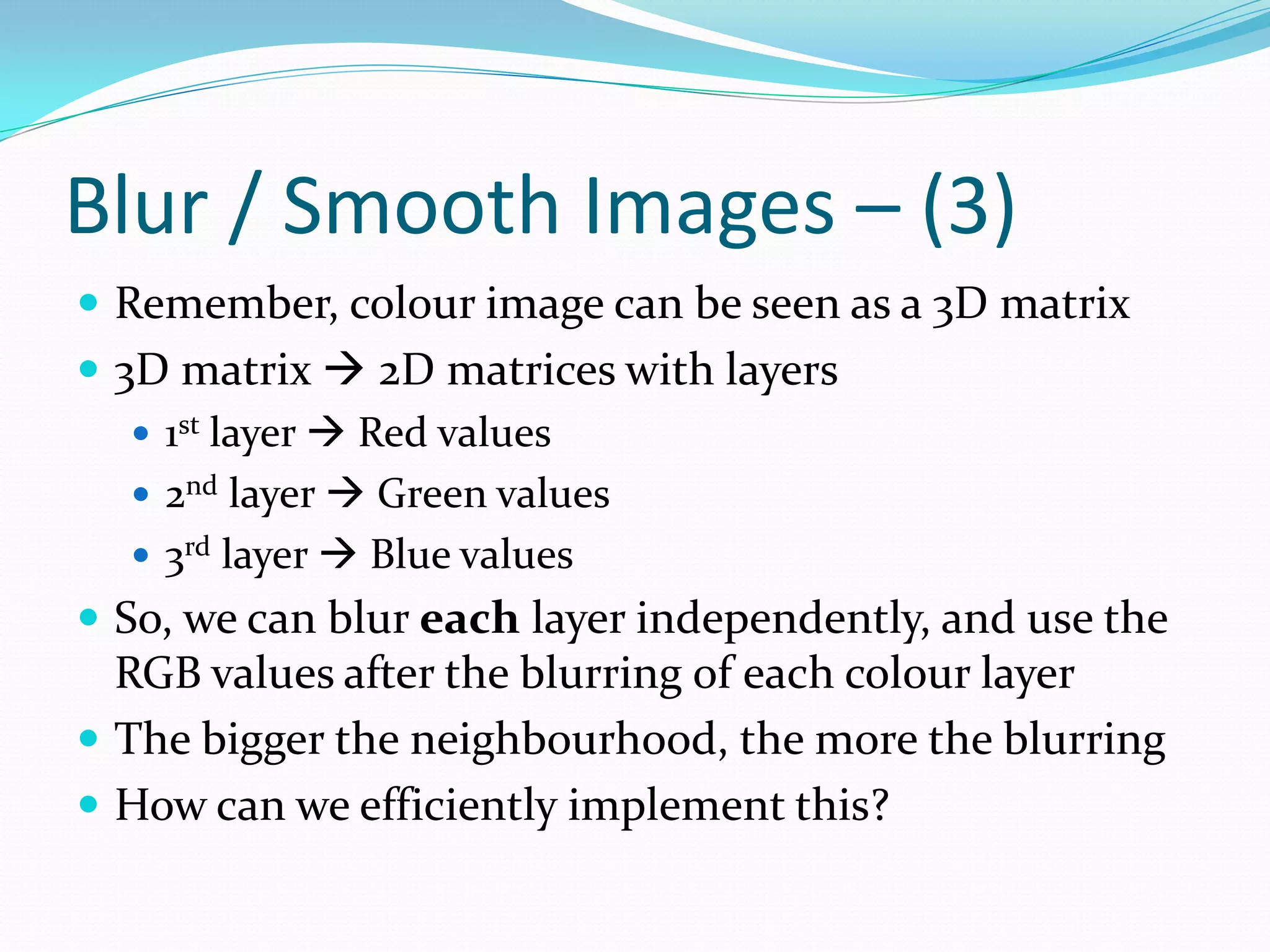
![Intro to Digital Images – (3) Monochromatic Case: We call the values at each pixel intensities Smaller intensities denote a darker pixel Bigger intensities denote a lighter pixel Colour Case: Think of a colour image as a 3D matrix First layer is red, second layer is green, third layer is blue Why RGB? Trichromacy theory All colours found in nature can naturally be decomposed into Red, Green and Blue This is basically how CCD cameras work! The three element vector tells you how much red, green and blue the pixel is compromised of (i.e. [R G B]T = [0 255 0] No red, no blue, all green](https://image.slidesharecdn.com/ieeediptalkf2011-120903013148-phpapp02/75/Introduction-to-Digital-Image-Processing-Using-MATLAB-14-2048.jpg)
![Intro to Digital Images – (4) Pixel : [ p, I(p)] p = (r, c ) red 12 Pixel Location: p = (r , c) = (row # , col # ) I ( p ) = green = 43 Pixel Value: I(p) = I(r , c) = (272, 277) blue 61 ](https://image.slidesharecdn.com/ieeediptalkf2011-120903013148-phpapp02/75/Introduction-to-Digital-Image-Processing-Using-MATLAB-15-2048.jpg)
![R/W Images in MATLAB – (4) So I know how to get pixels; how can I modify them in the image? Easy! Just go backwards For a B & W Image do: im(row,col) = pix; For a colour image, do either: im(row,col,1) = red; im(row,col,2) = green; im(row,col,3) = blue; or im(row,col,:) = [red; green; blue] or im(row,col,:) = rgb; %rgb - 3 x 1 vector](https://image.slidesharecdn.com/ieeediptalkf2011-120903013148-phpapp02/75/Introduction-to-Digital-Image-Processing-Using-MATLAB-25-2048.jpg)
![R/W Images in MATLAB – (6) So I know how to get pixels; how can I display images? Use the imshow() command imshow(im); im: Image loaded into MATLAB Shows a new window with the image in it If you do: imshow(im,[]) For monochromatic: Smallest intensity becomes 0 and largest intensity becomes 255 for display For colour: Apply the above for each colour channel Every time you use imshow, the image you want to display is put in the same window… so what do you do?](https://image.slidesharecdn.com/ieeediptalkf2011-120903013148-phpapp02/75/Introduction-to-Digital-Image-Processing-Using-MATLAB-27-2048.jpg)
![Resizing Images One common thing that many people do is resize images i.e. Make an image bigger from a smaller image, or make an image smaller from a larger image How do we resize images in MATLAB? Use the imresize command How do we use it? out = imresize(im, scale, ‘method’); or out = imresize(im, [r c], ‘method’); For both methods im is the image we want to resize, and out is the resized image](https://image.slidesharecdn.com/ieeediptalkf2011-120903013148-phpapp02/75/Introduction-to-Digital-Image-Processing-Using-MATLAB-32-2048.jpg)
![Resizing Images – (4) Now, let’s take a look at the second method for resizing out = imresize(im, [r c], ‘method’); This routine will resize the image to any desired dimensions you want You can customize how many rows and columns the final image will have Example: To resize a 130 rows x 180 columns image to 65 rows x 90 columns, with bilinear interpolation, do: out = imresize(im, [65 90], ‘bilinear’); We can also do! out = imresize(im, 0.5, ‘bilinear’);](https://image.slidesharecdn.com/ieeediptalkf2011-120903013148-phpapp02/75/Introduction-to-Digital-Image-Processing-Using-MATLAB-35-2048.jpg)
![Cont. & Brig. Enhancement (4) How do we apply the power law in MATLAB? Use imadjust out = imadjust(im, [], [], gamma); im: Input image to contrast adjust Ignore 2nd and 3rd parameters Beyond the scope of our talk gamma: The γ exponent that we’ve seen earlier out: The contrast adjusted image Example use: If γ = 1.4, we do: out = imadjust(im, [], [], 1.4);](https://image.slidesharecdn.com/ieeediptalkf2011-120903013148-phpapp02/75/Introduction-to-Digital-Image-Processing-Using-MATLAB-42-2048.jpg)
![Intro to Image Histograms We can perform more advanced image enhancement using histograms Before we cover this… we should probably cover what histograms are! So, what’s a histogram? It measures the frequency, or how often, something occurs Let’s look at a grayscale image for now Expressed as H(x) = q, x is an intensity- [0,255] for 8 bits This tells us that we see the intensity value of x for a total of q times](https://image.slidesharecdn.com/ieeediptalkf2011-120903013148-phpapp02/75/Introduction-to-Digital-Image-Processing-Using-MATLAB-45-2048.jpg)


![Edge Detection – (8) Any gradient value < 128 is labelled black thresh is between [0,1], so take your threshold and divide by 255 to use i.e. I = edge(im, ‘prewitt’, 128/255); Output image will give you a black and white image White is an edge, black is not an edge Only works for B & W images. To find edges for colour images, convert the colour image to a B & W image Use gray = rgb2gray(im); rgb2gray converts a colour image into B & W by doing: I = (R + G + B) / 3 Each colour pixel is the average of the red, green and blue components](https://image.slidesharecdn.com/ieeediptalkf2011-120903013148-phpapp02/75/Introduction-to-Digital-Image-Processing-Using-MATLAB-81-2048.jpg)
![Noise Filtering – (4) For each pixel (r,c) in the image, extract an M x N subset of pixels centered at (r,c) Sort these pixels in ascending order, and grab the median value The output image at (r,c) is this value How do we perform median filtering in MATLAB? out = medfilt2(im, [M N]);](https://image.slidesharecdn.com/ieeediptalkf2011-120903013148-phpapp02/75/Introduction-to-Digital-Image-Processing-Using-MATLAB-97-2048.jpg)
![Template Matching – (3) Output is a correlation map To find the row and column co-ordinates of where the template best matches, do the following: [row col] = find(C == max(C(:))); So, how do we do image stitching? 1) Extract a region in either image that is common between both Template 2) Find the co-ordinates of where this template is in both images 3) Determine how much vertical and horizontal displacement there is between the two images](https://image.slidesharecdn.com/ieeediptalkf2011-120903013148-phpapp02/75/Introduction-to-Digital-Image-Processing-Using-MATLAB-102-2048.jpg)

The document is a presentation by Ph.D. candidate Raymond Phan on digital image processing using MATLAB, covering topics such as basic image manipulation, pixel access, and image enhancement techniques. It discusses the structure of digital images, including color representation, basic MATLAB commands for image I/O, and image resizing methods, complemented by personal background and research interests of the presenter. The presentation aims to provide foundational knowledge for working with digital images in MATLAB, including practical demonstrations and resources for further learning.
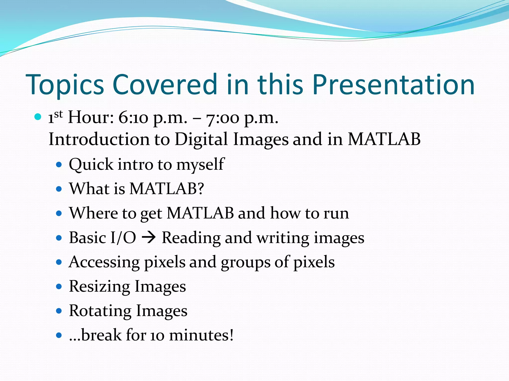
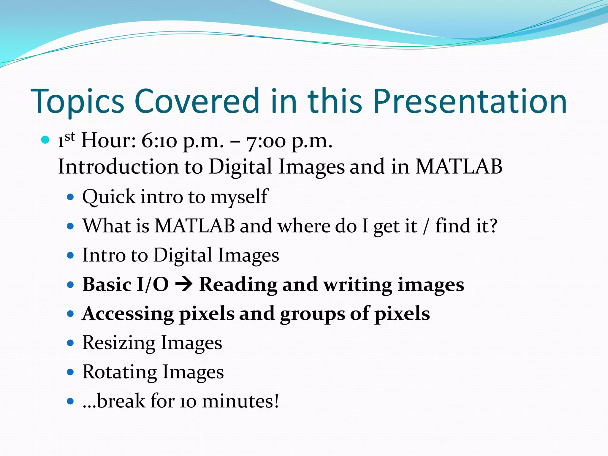
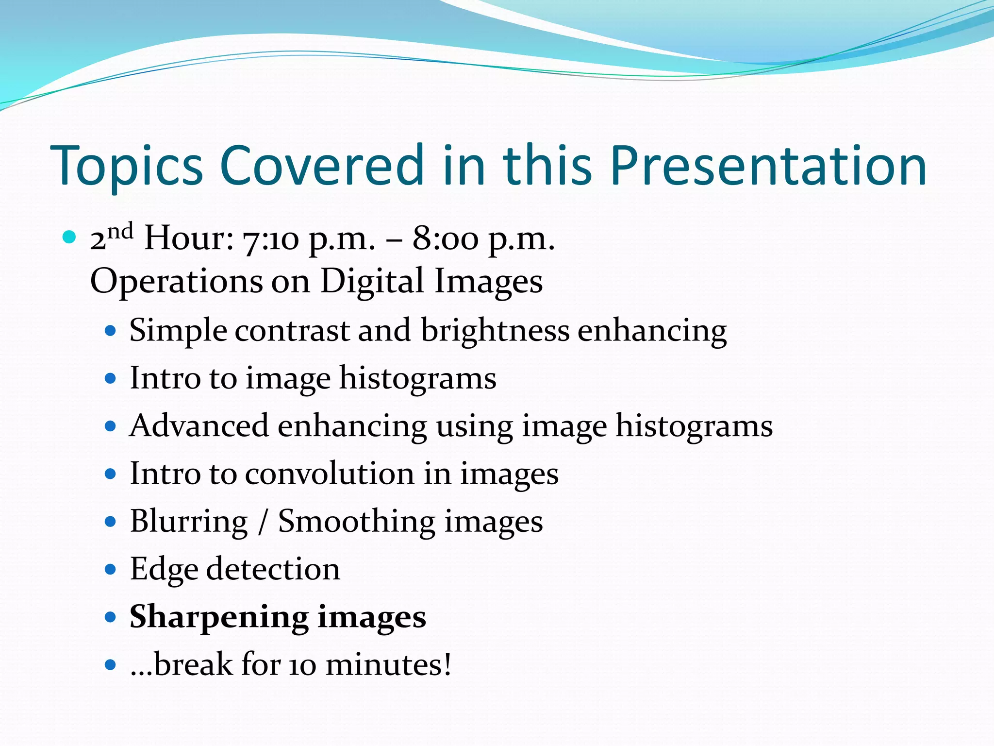
Introduction of the speaker and overview of the topics covered in the workshop including image processing and MATLAB.
Ph.D. Candidate introduction, academic journey, research interests, and achievements relating to digital image processing.
Explanation of MATLAB, installation options, and primary functionalities including Image Processing Toolbox.
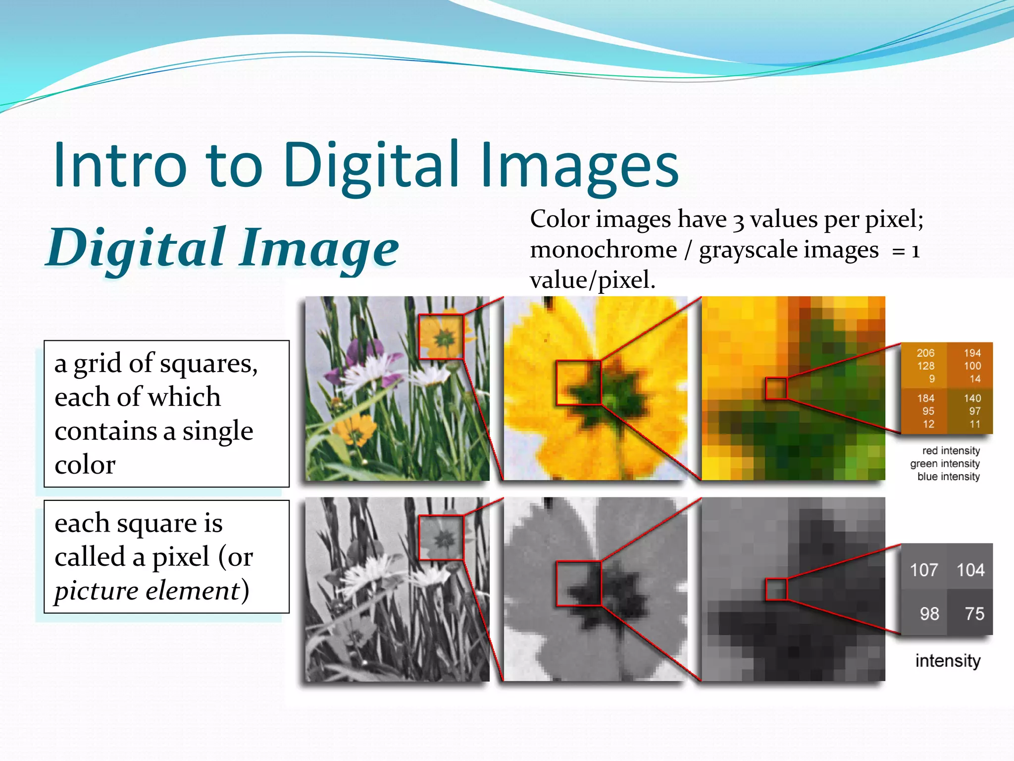
Introduction to digital images, pixel representation, color models, and basics of image capture.
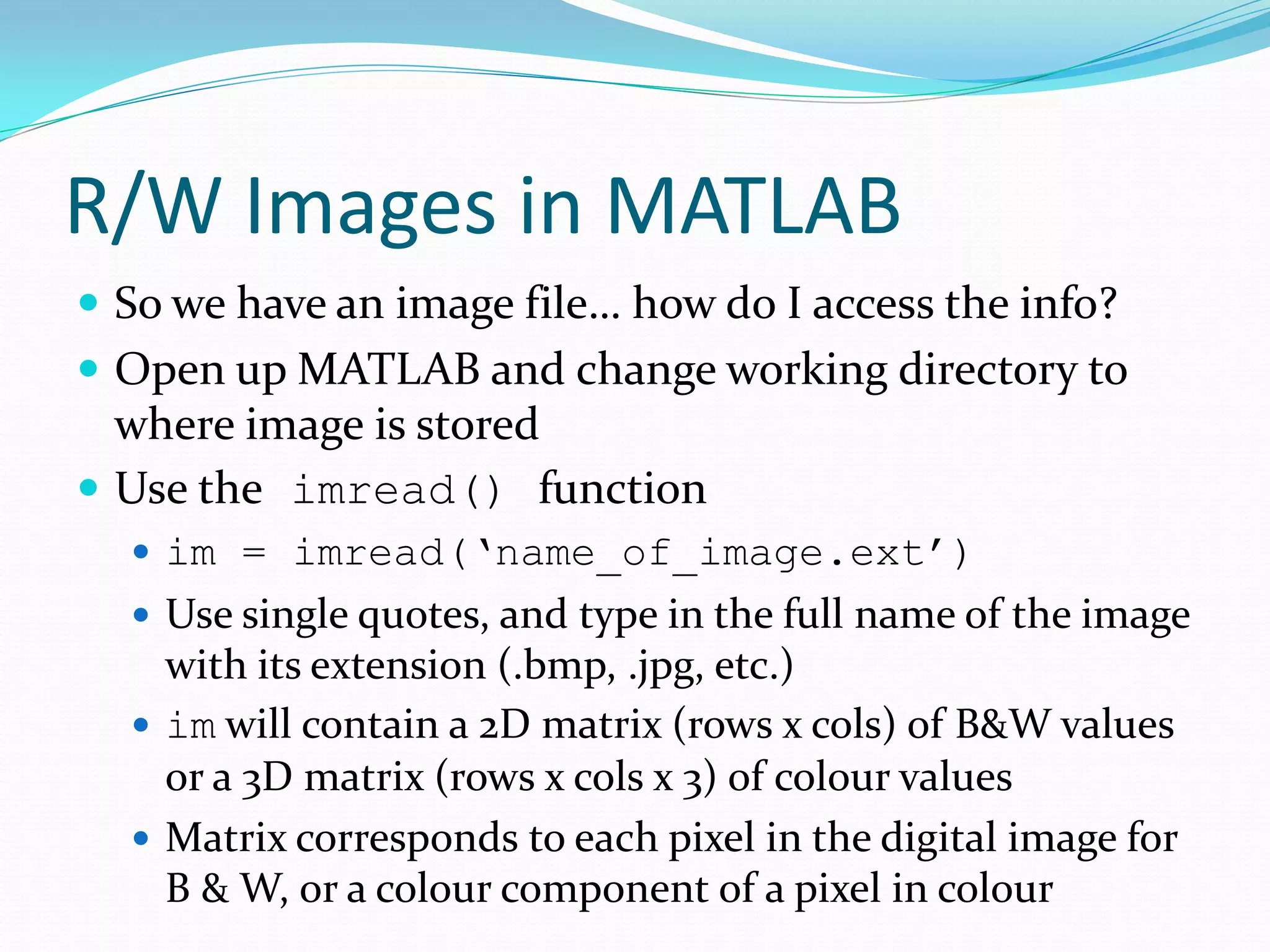
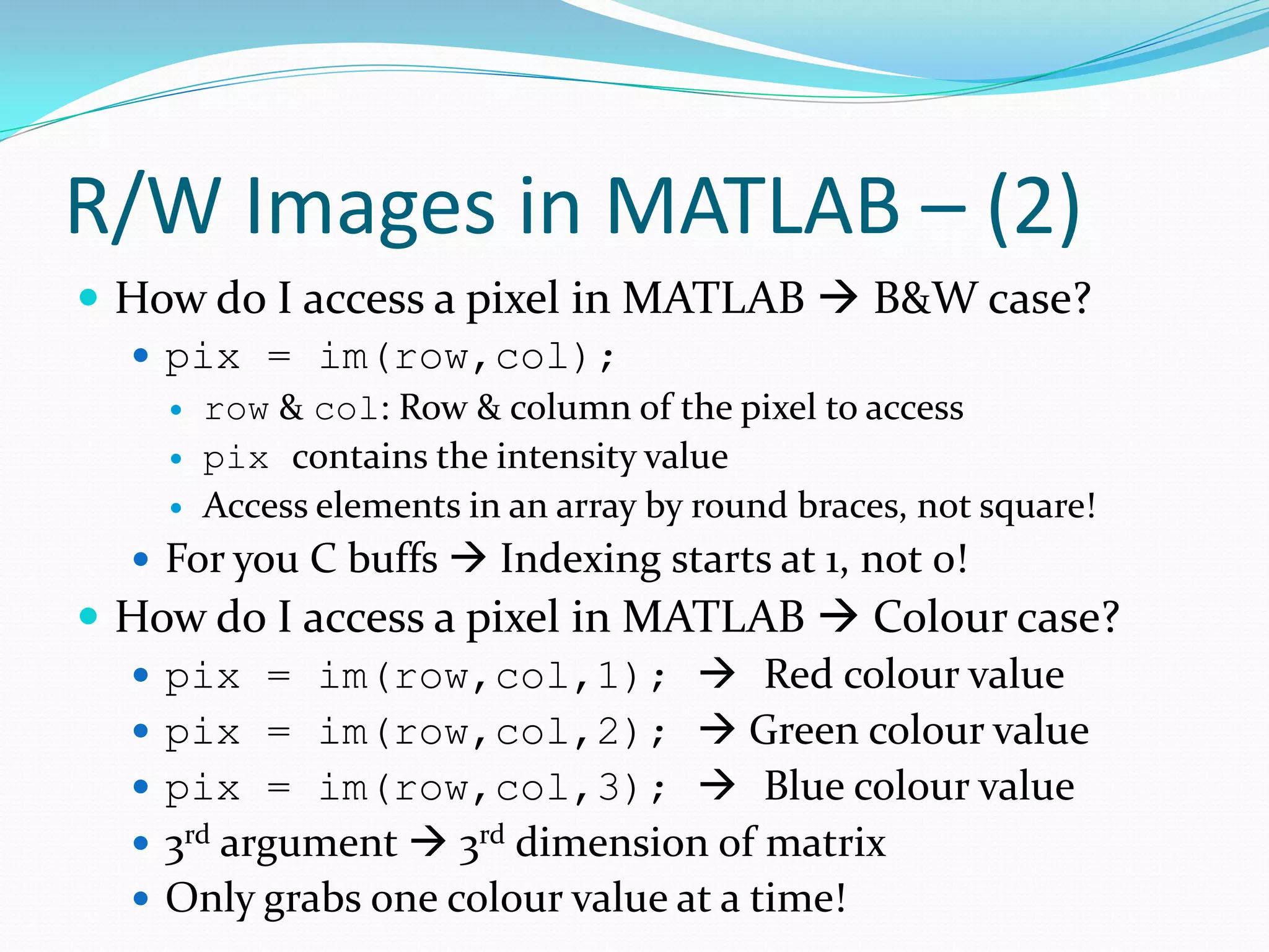
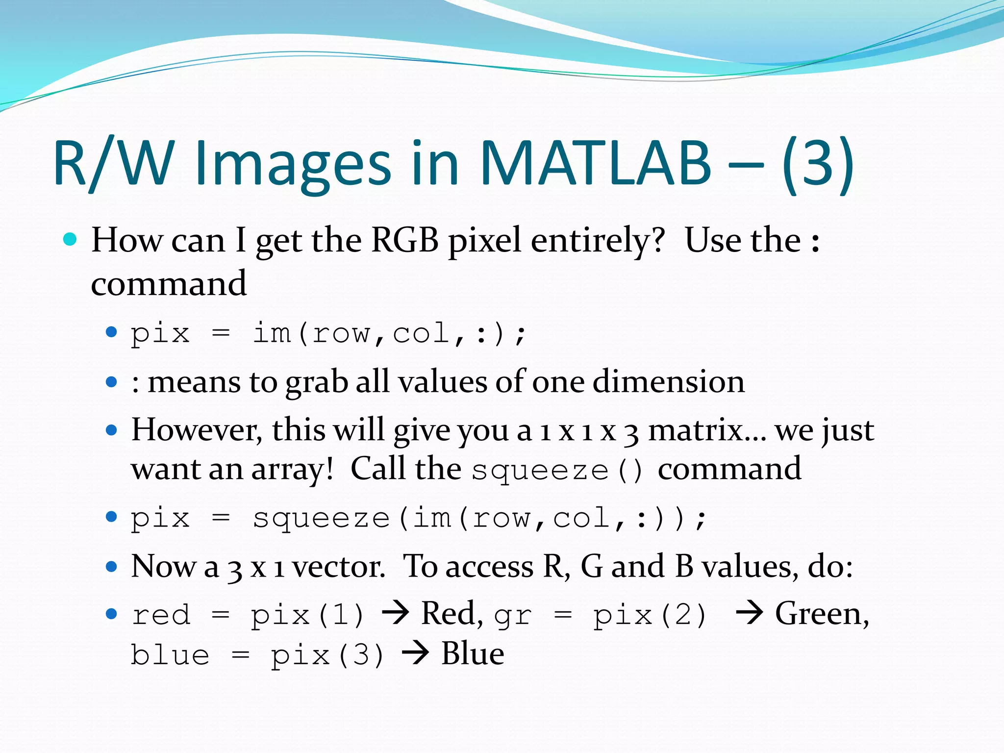
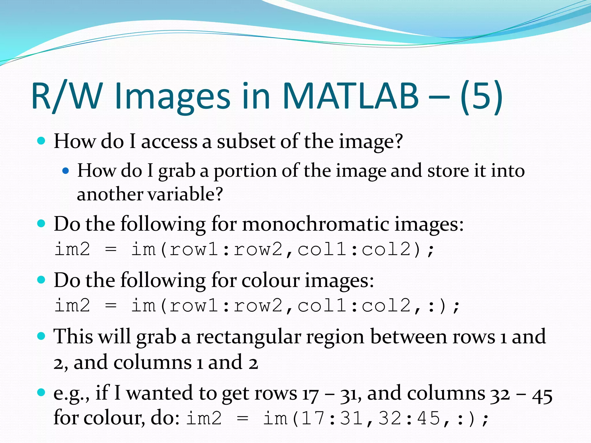
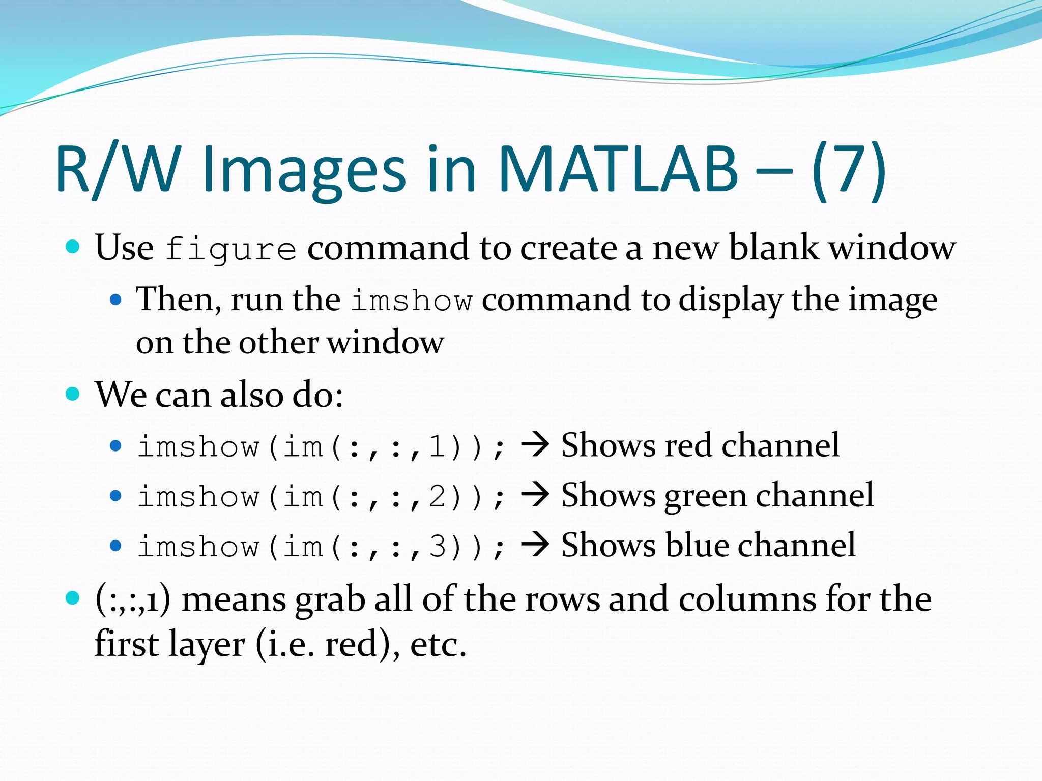
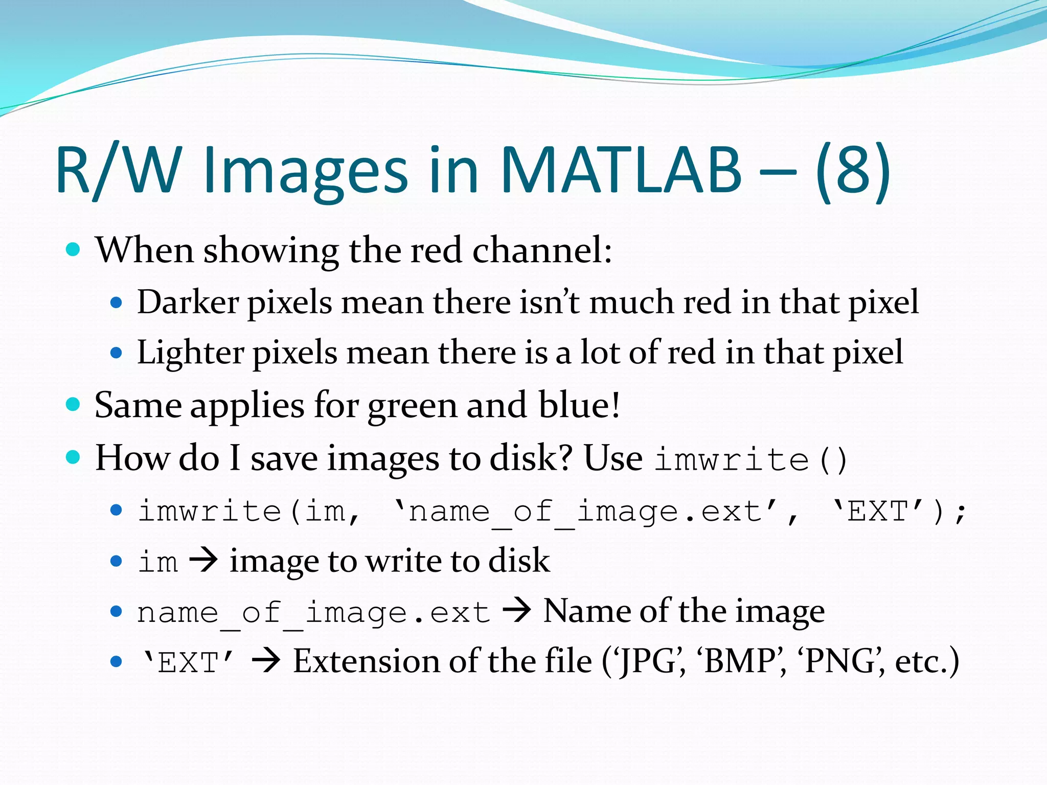
Procedures for reading, accessing, modifying pixels, resizing, and displaying images in MATLAB.
Discusses resizing images using imresize function, interpolation methods, and the impact of interpolation techniques.
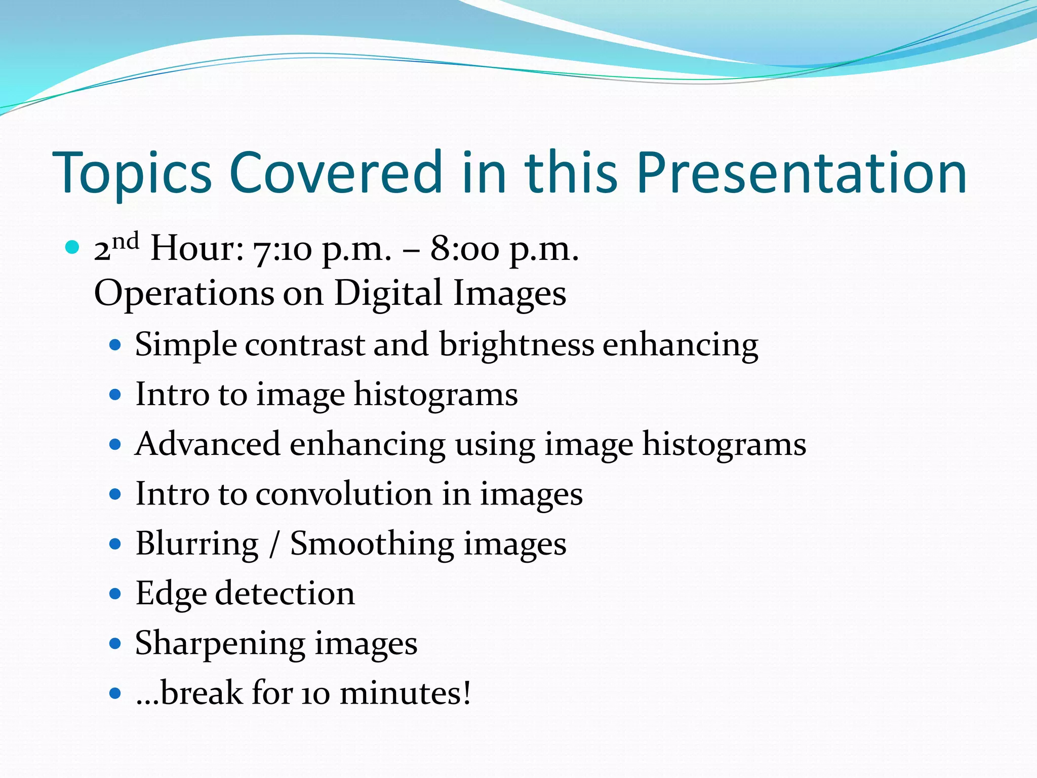
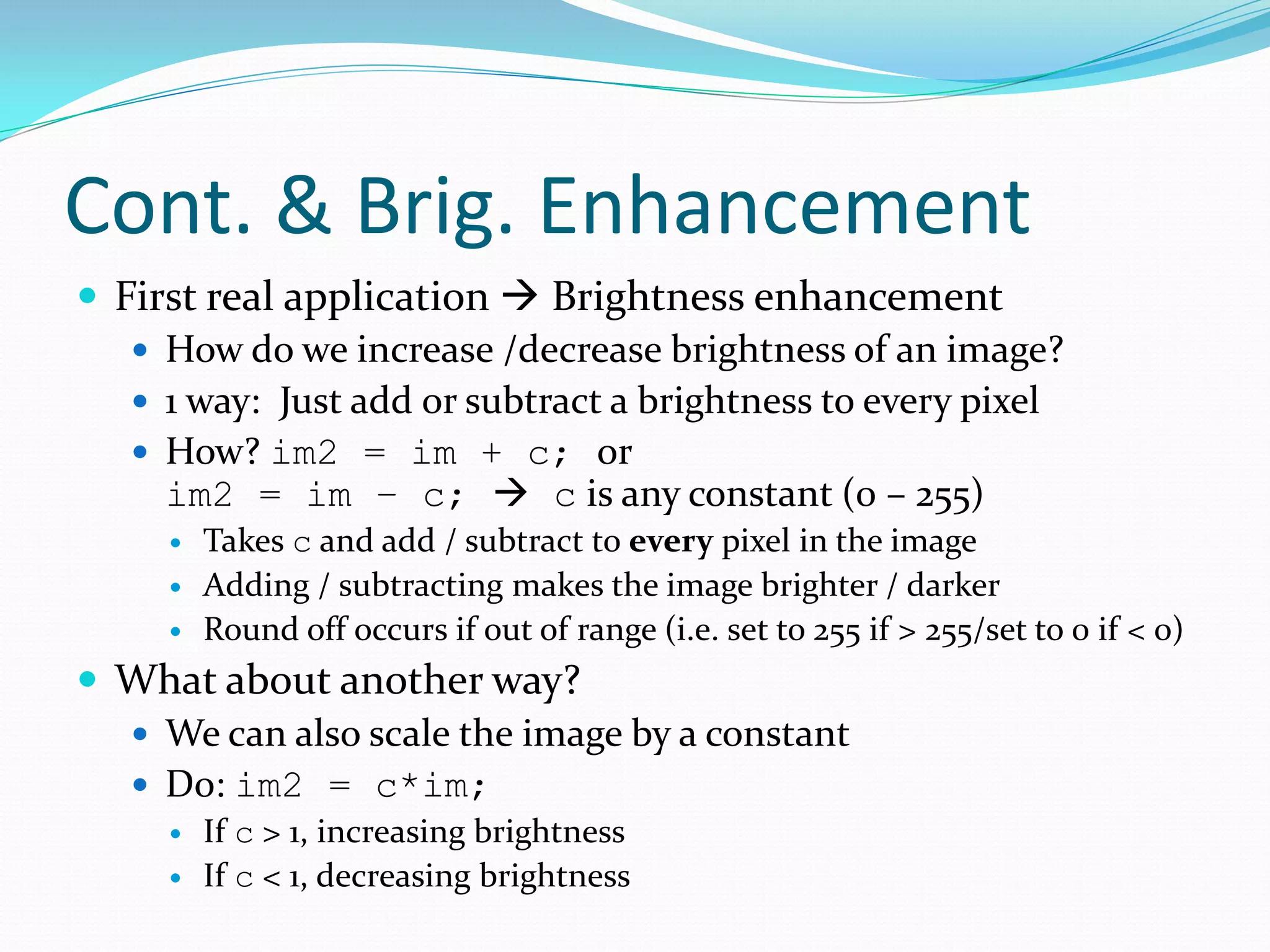
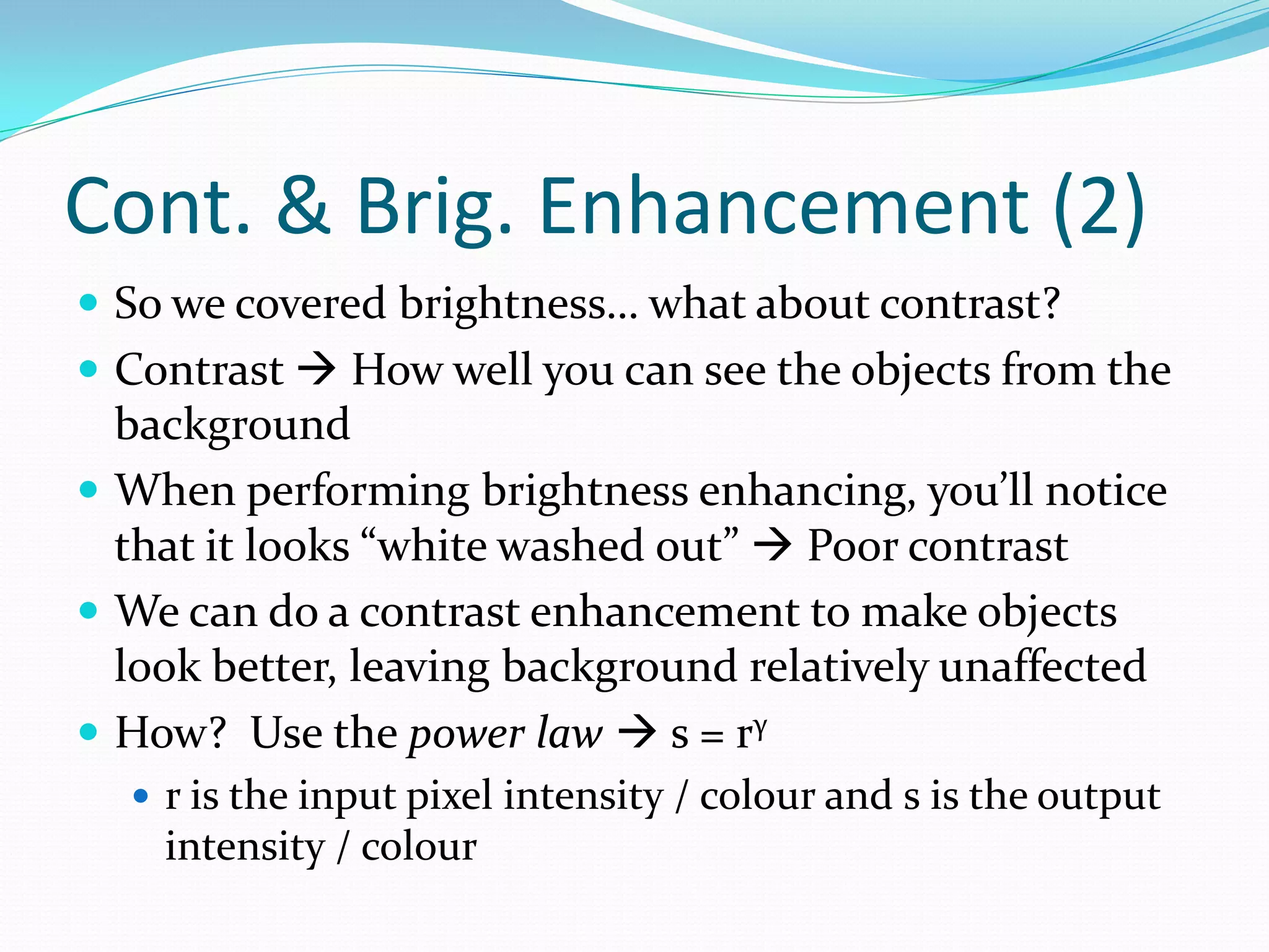
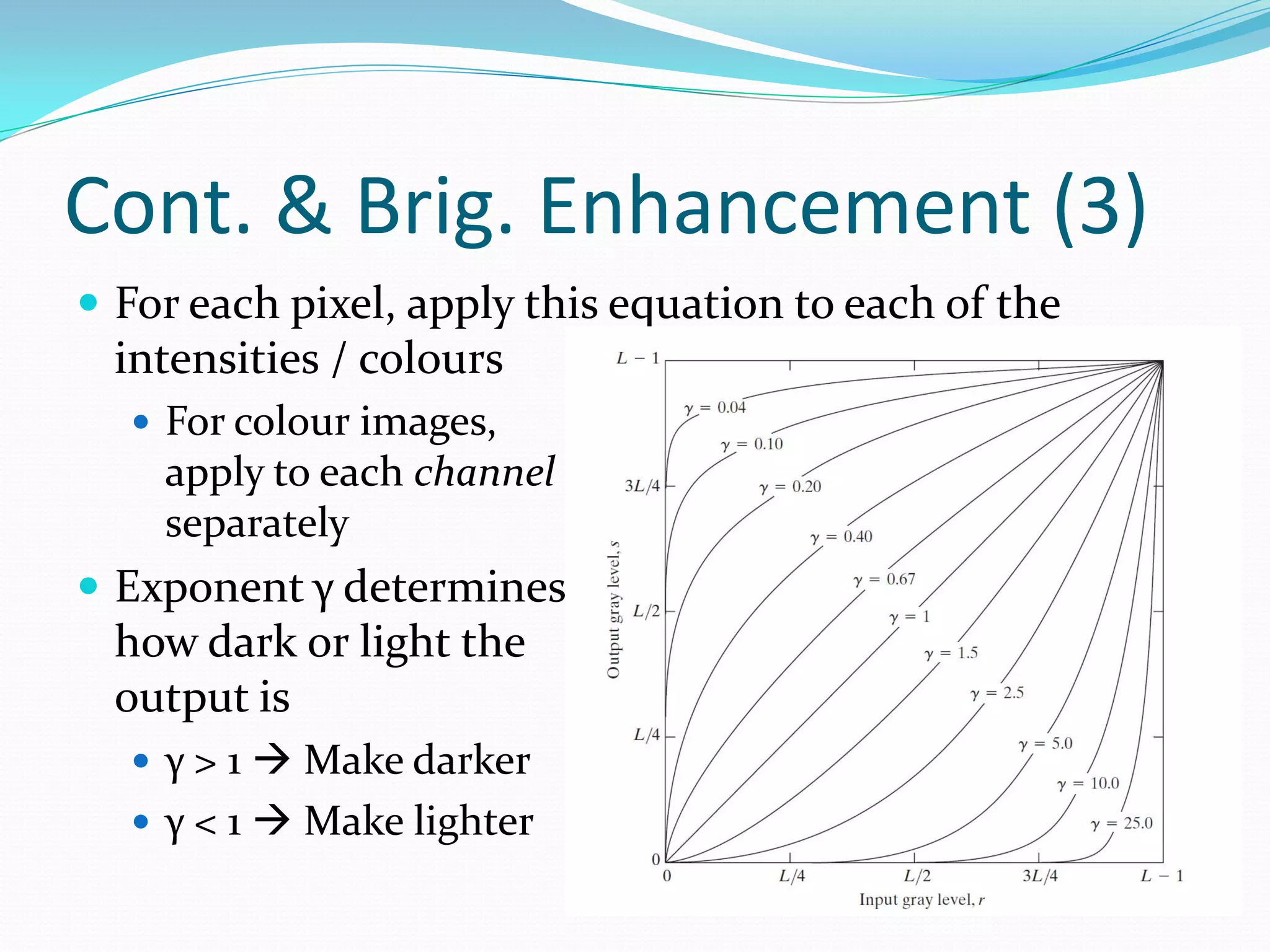
Techniques for adjusting brightness and contrast, including power law application for image enhancement.
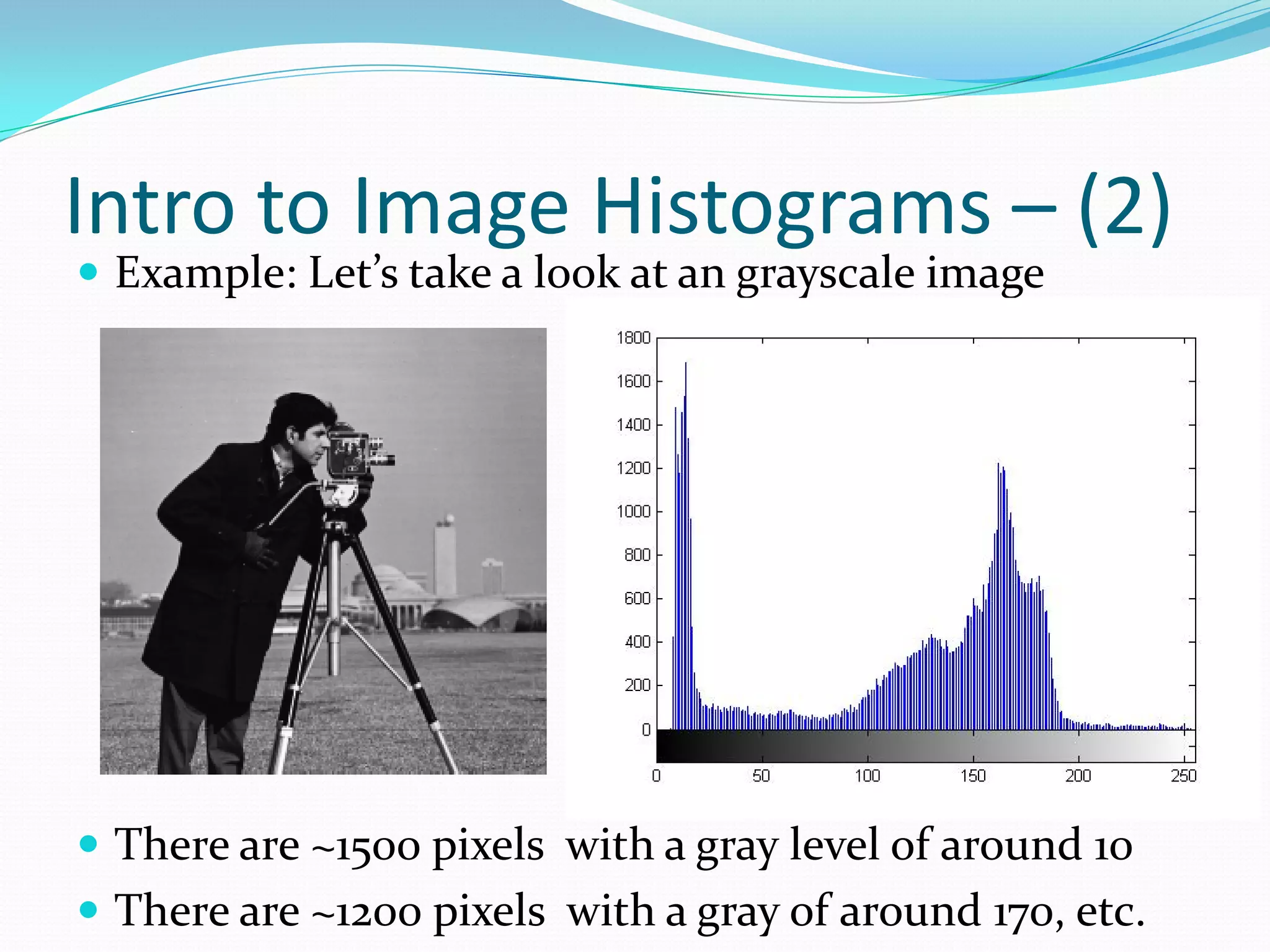
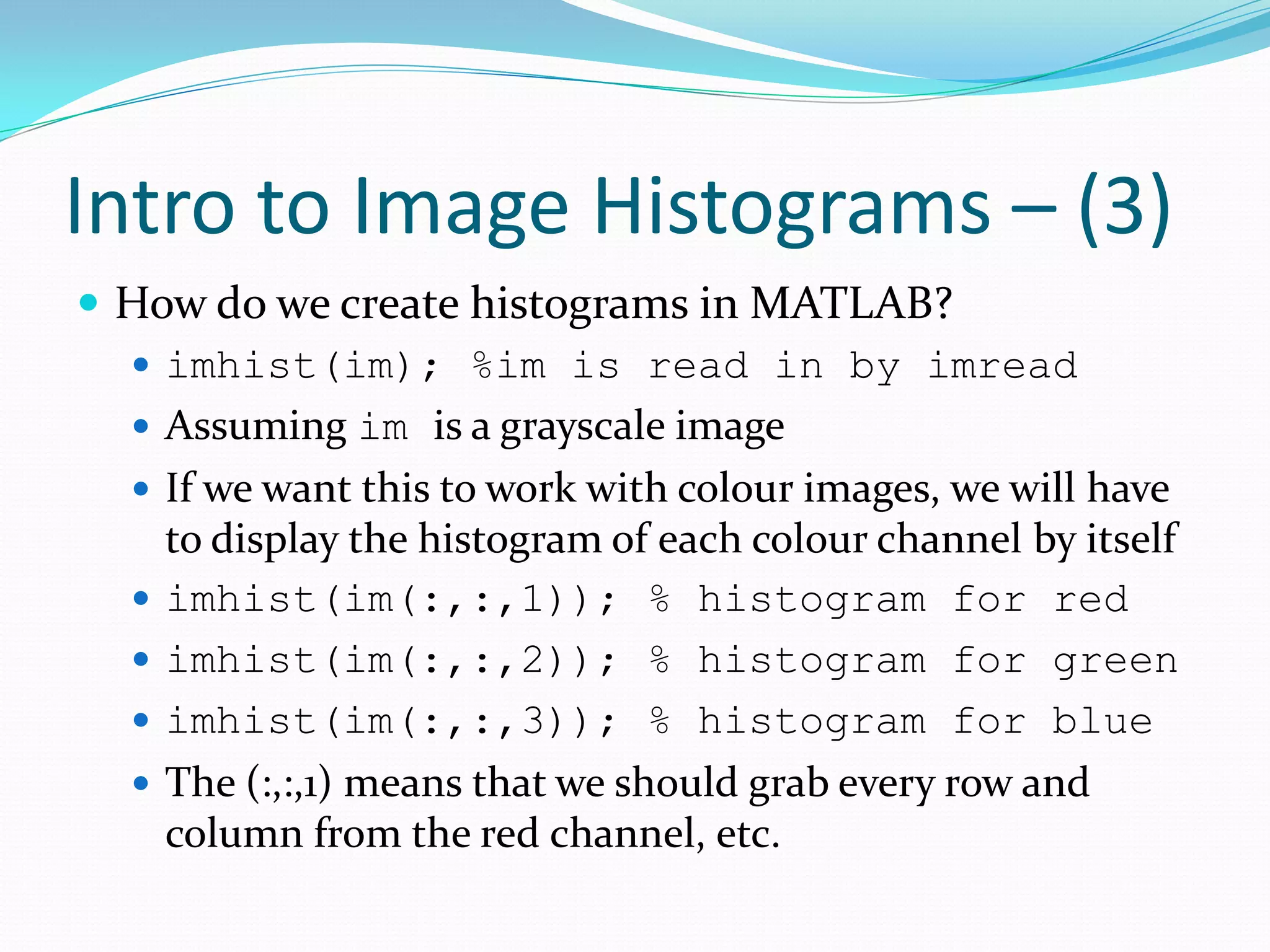
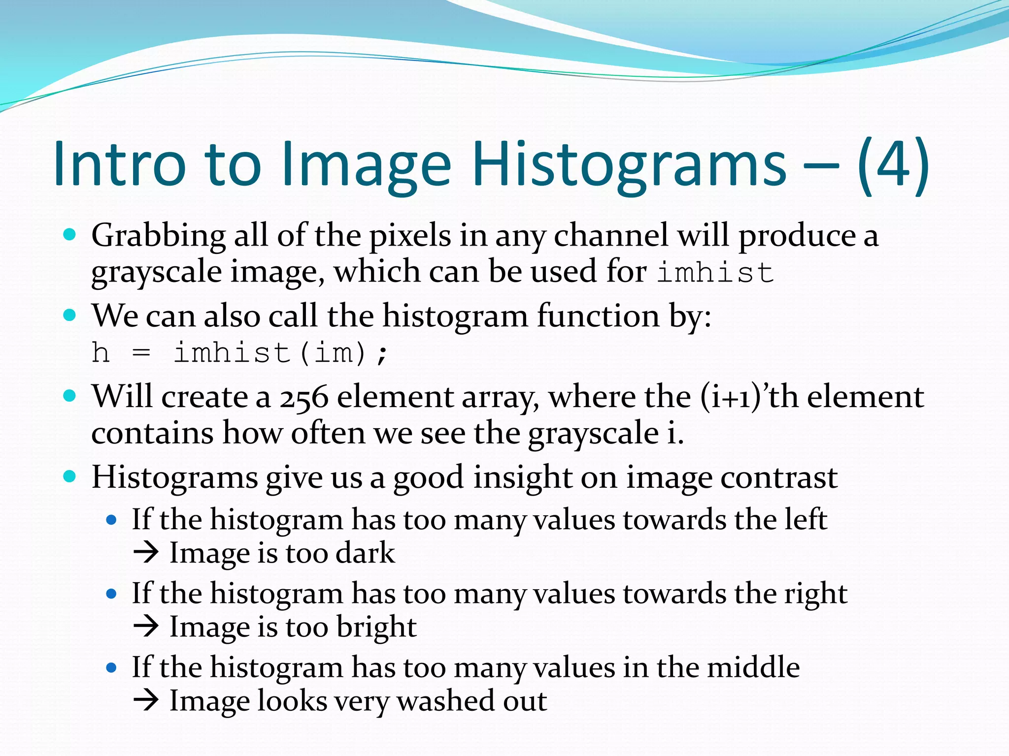
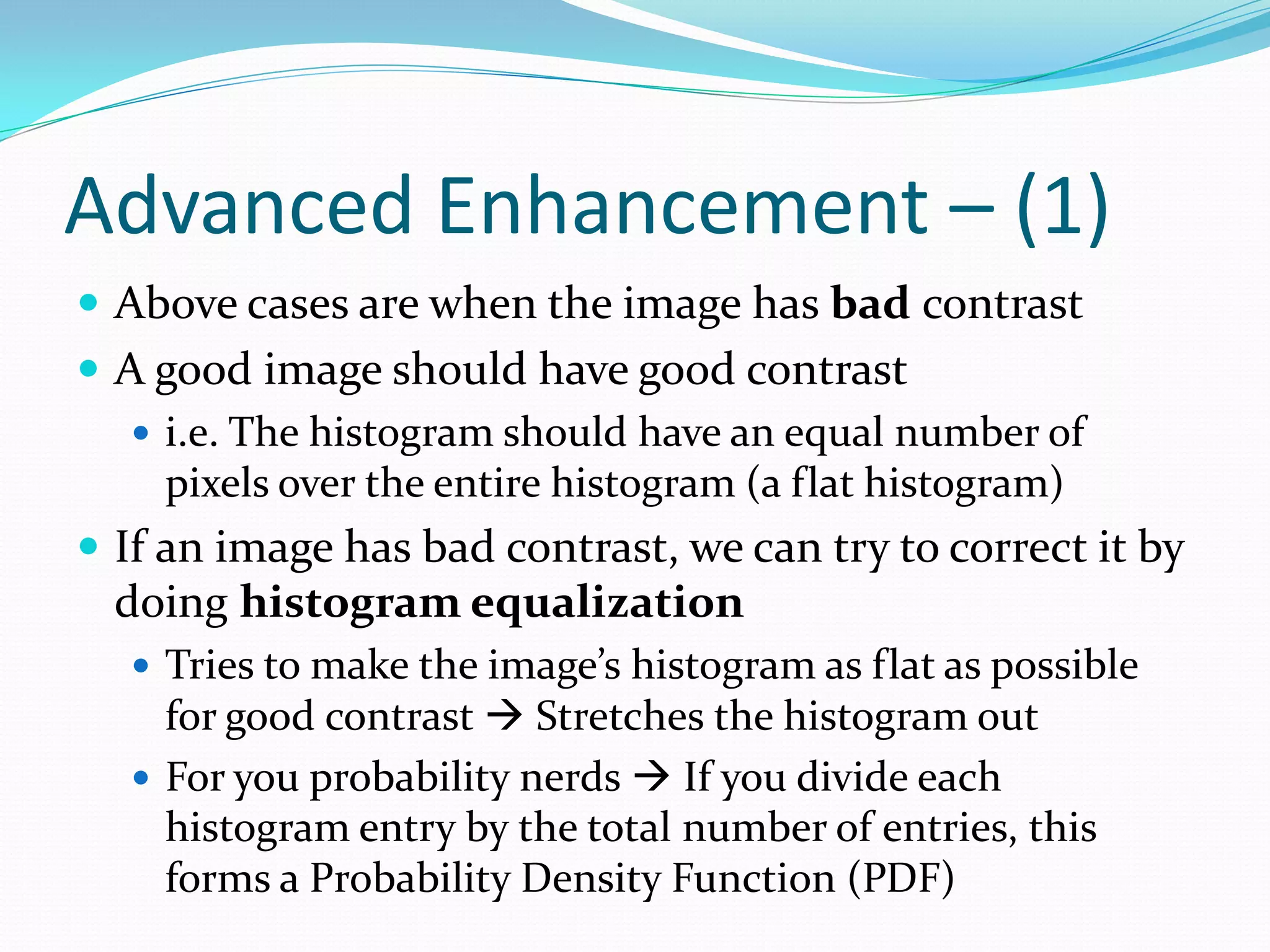
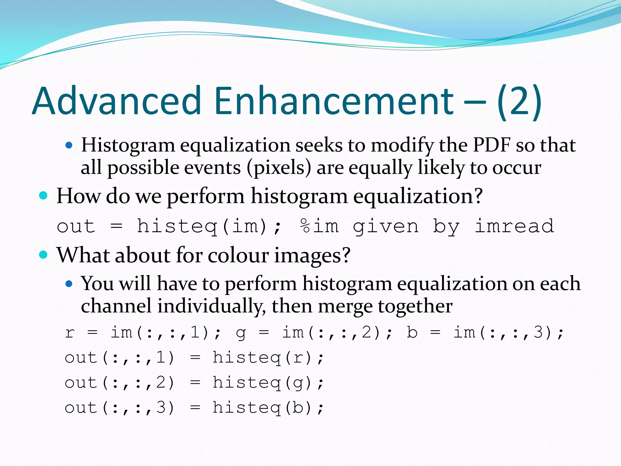
Introduction to histograms, their creation, and advanced techniques for image enhancement through histogram equalization.
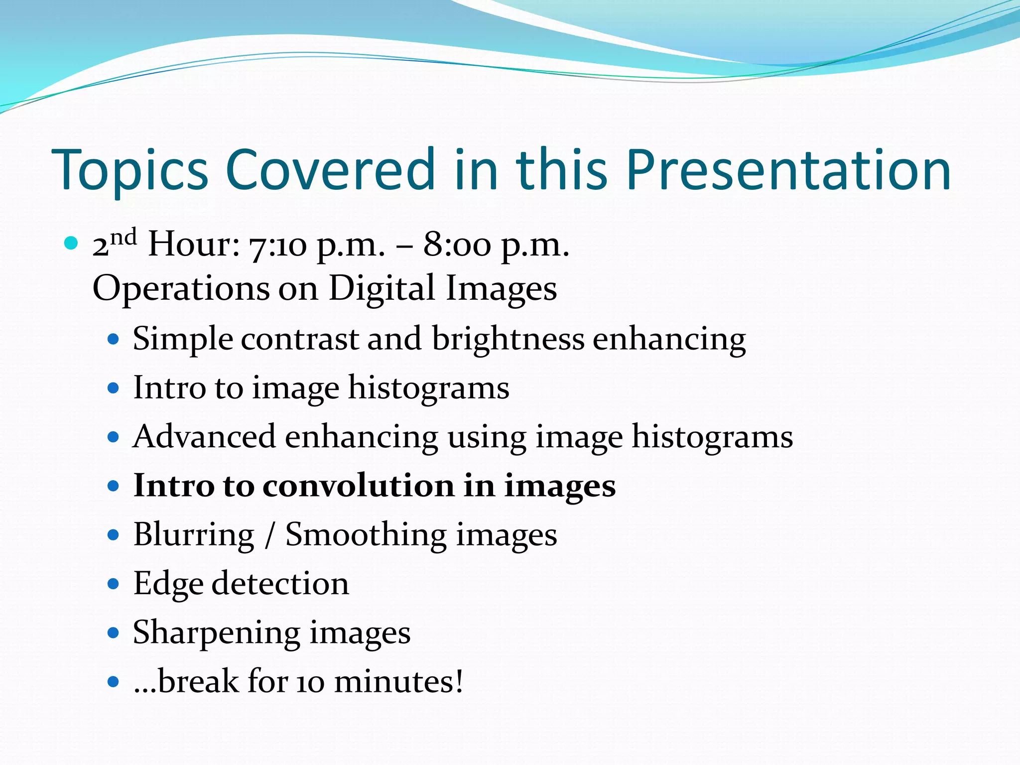
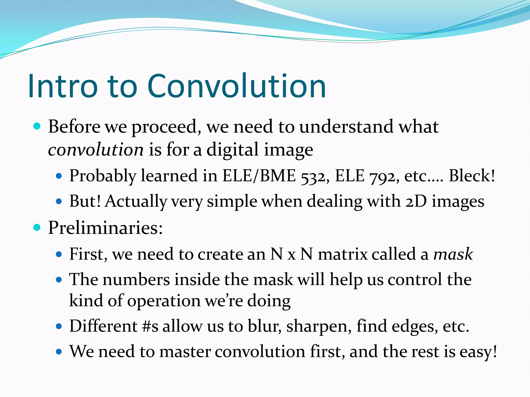
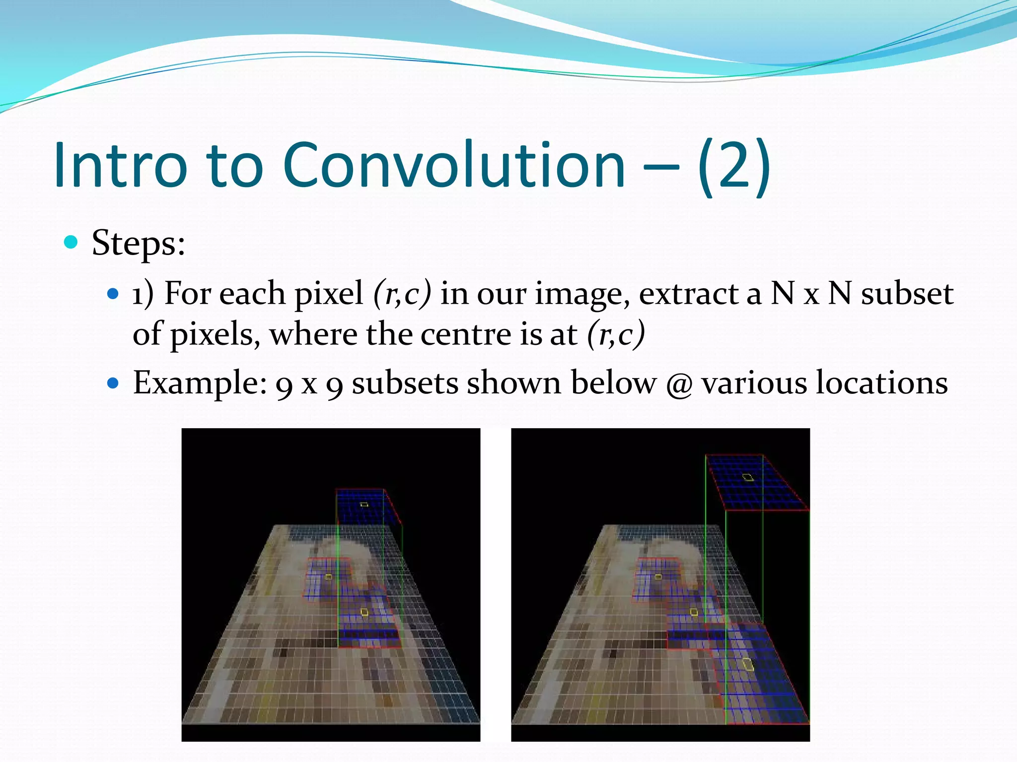
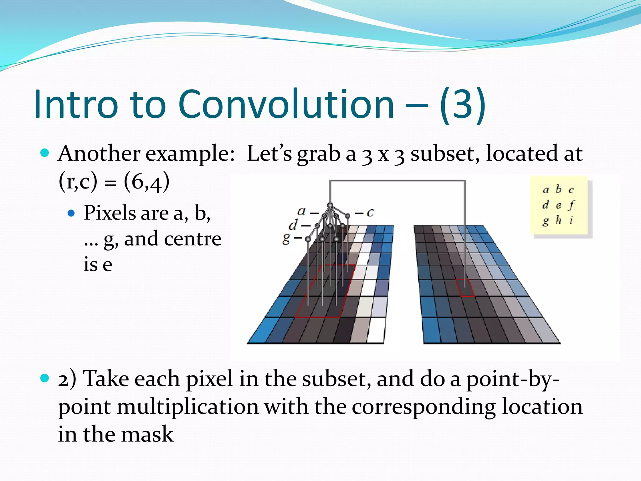
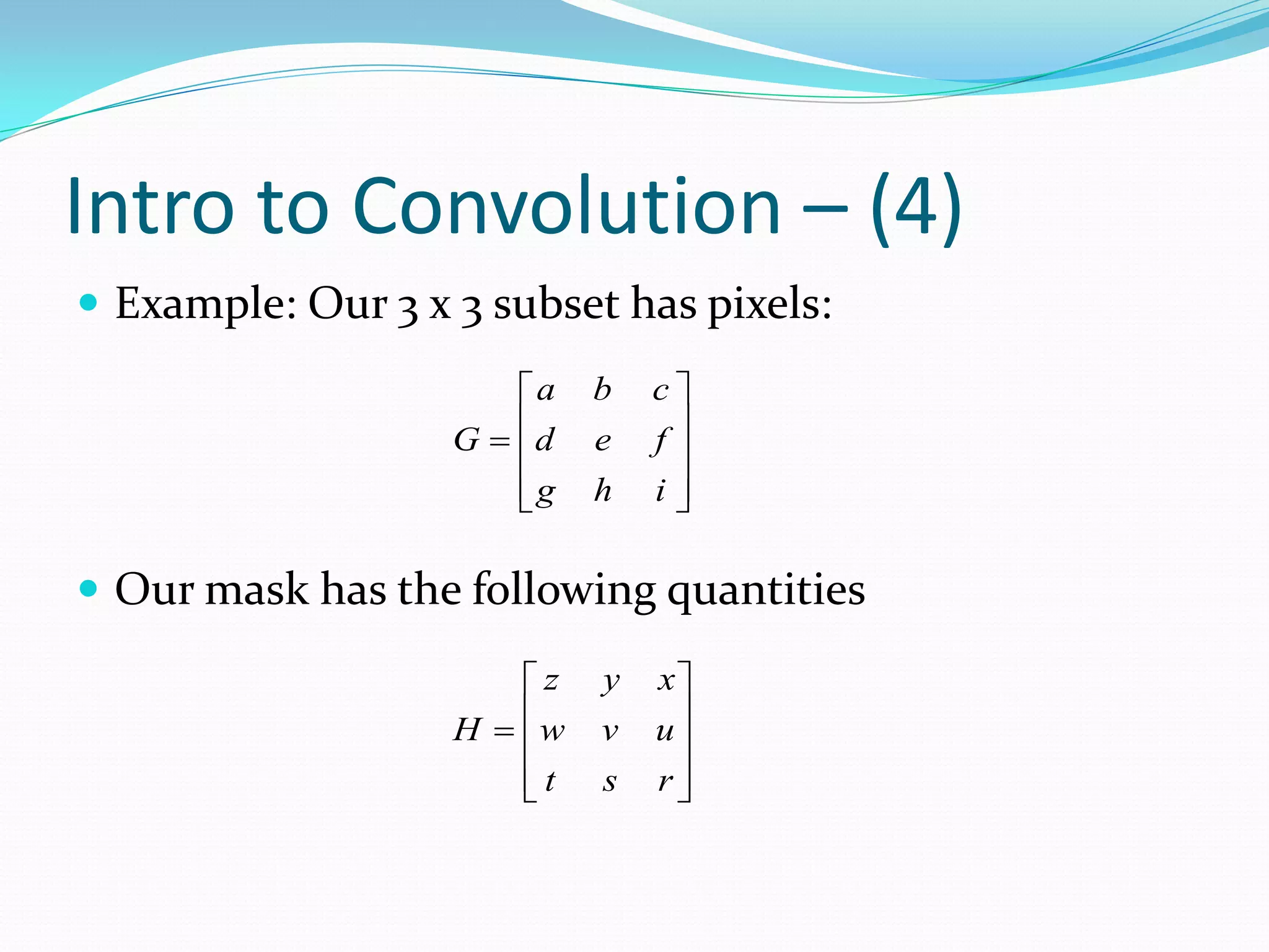
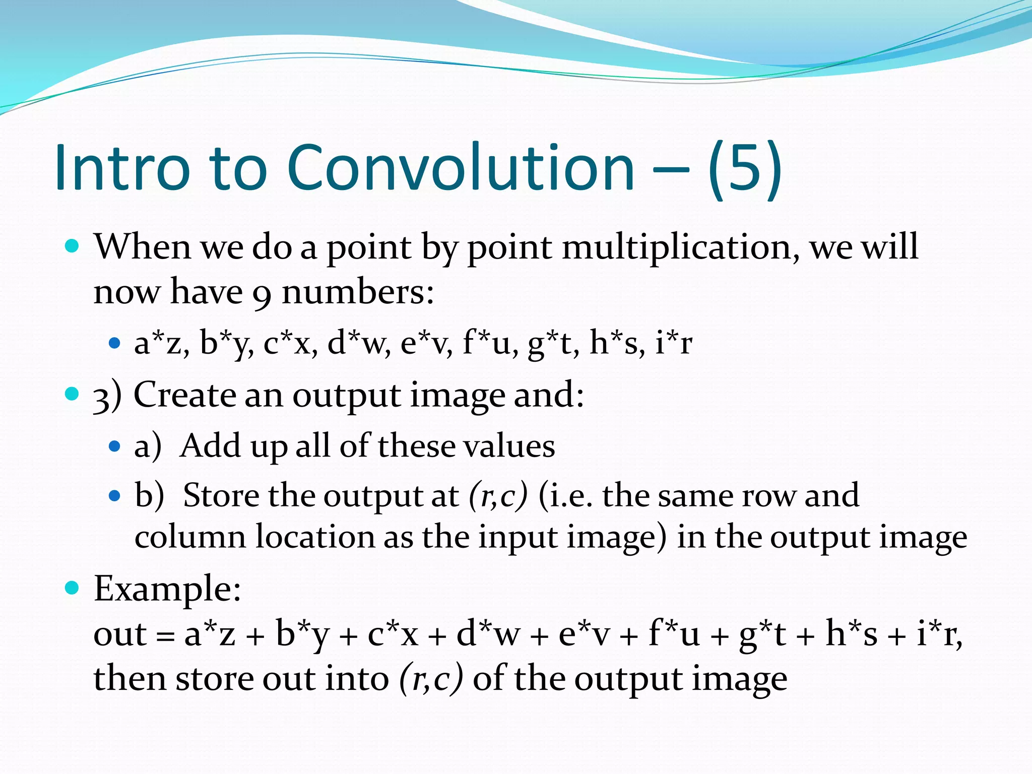
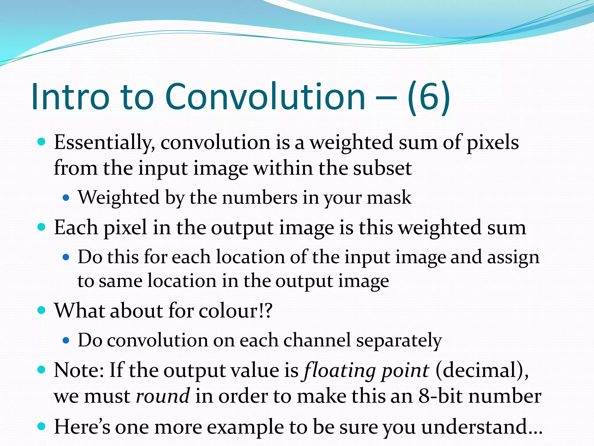
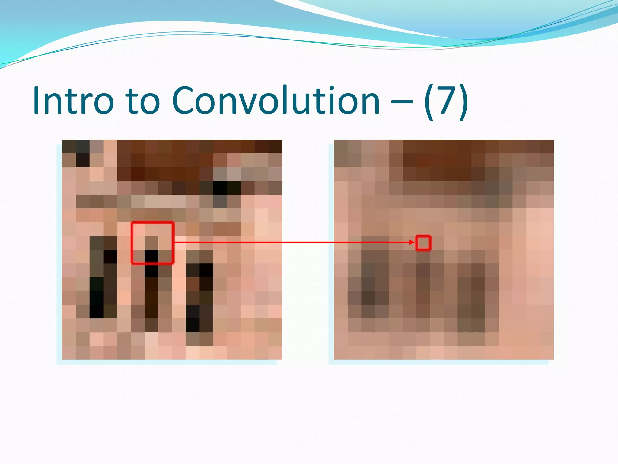
Introduction to convolution in 2D images, its mathematical foundation, and its applications in image filtering.
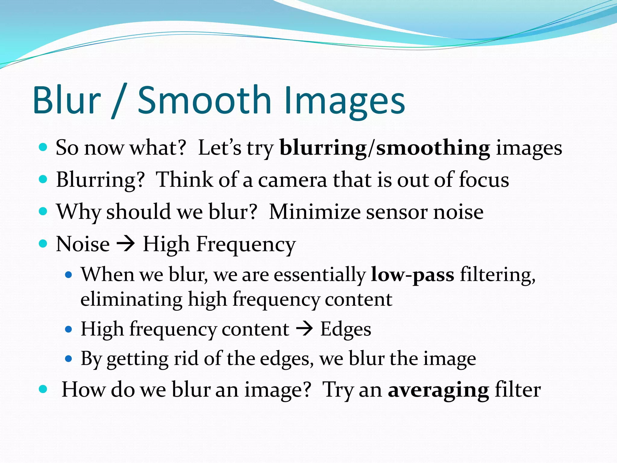
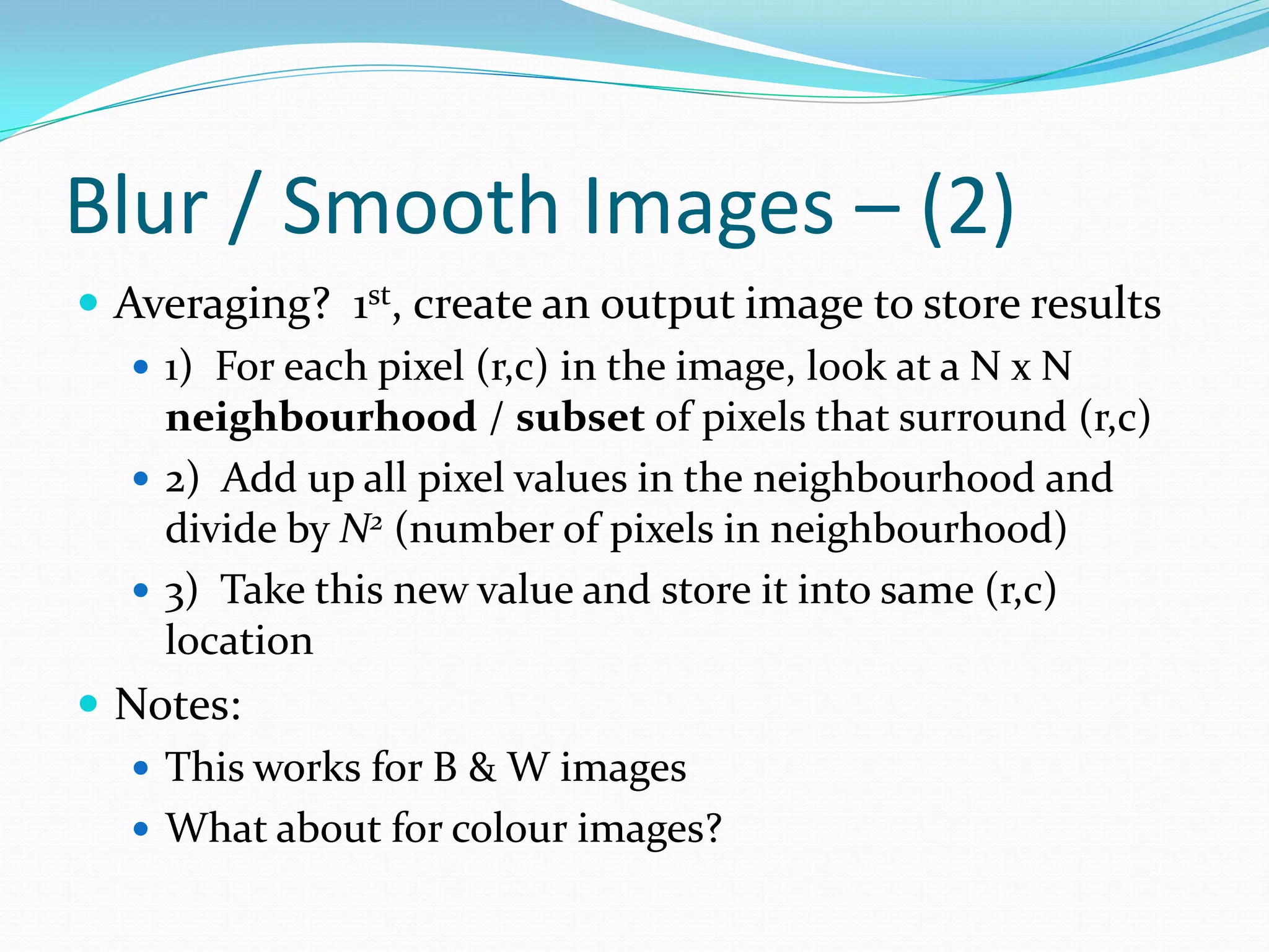
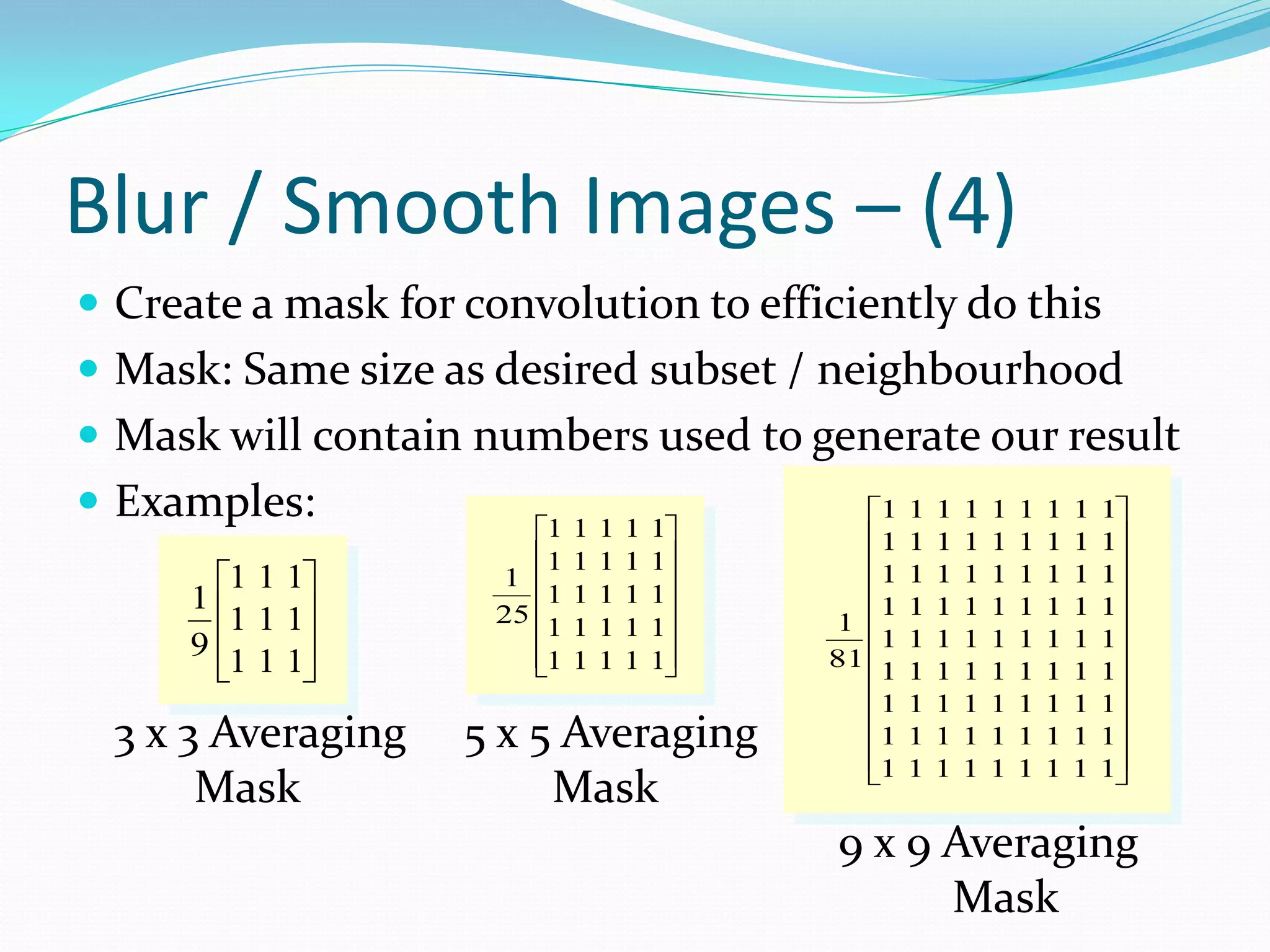
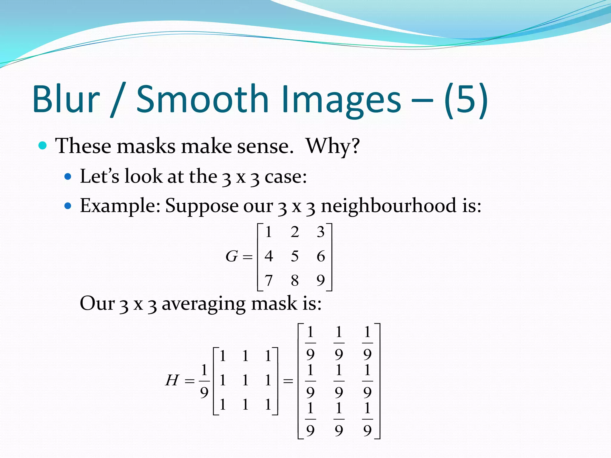
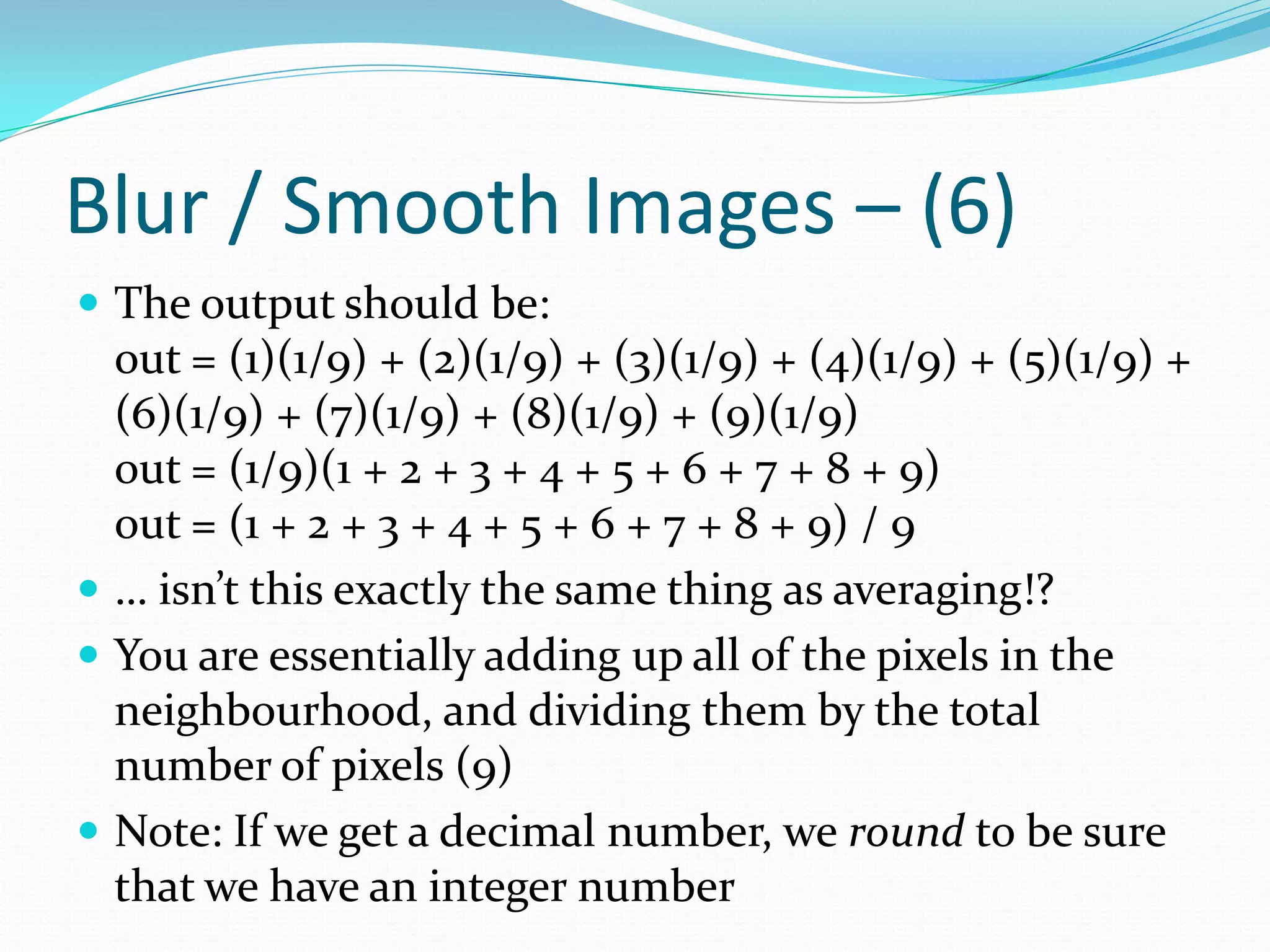
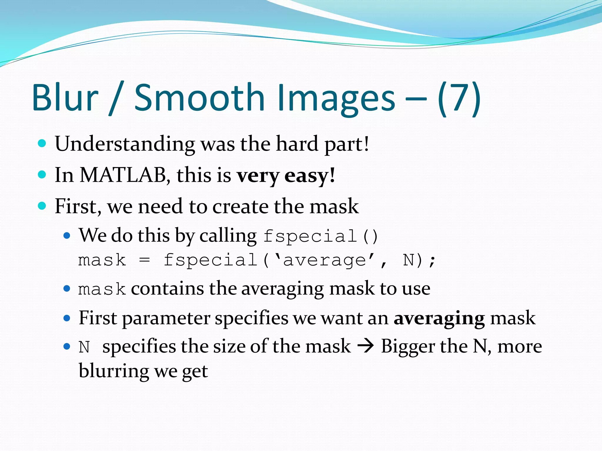
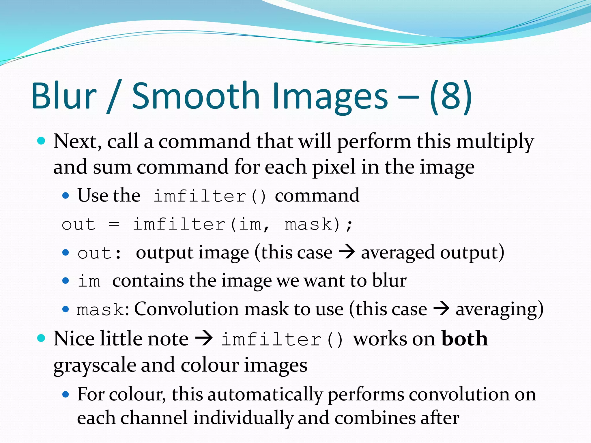
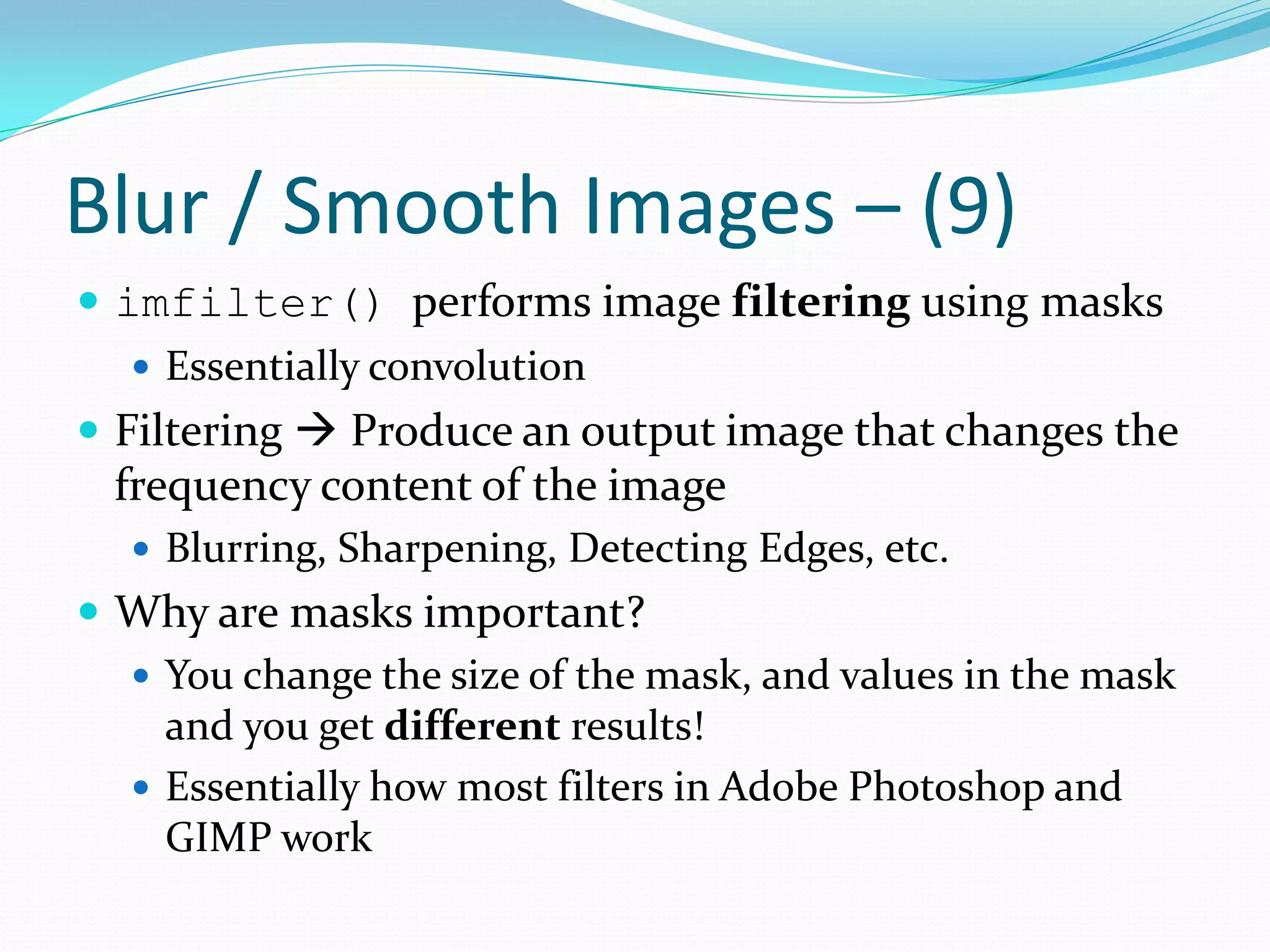
Techniques for blurring images using averaging filters, mask creation, and implementation in MATLAB.
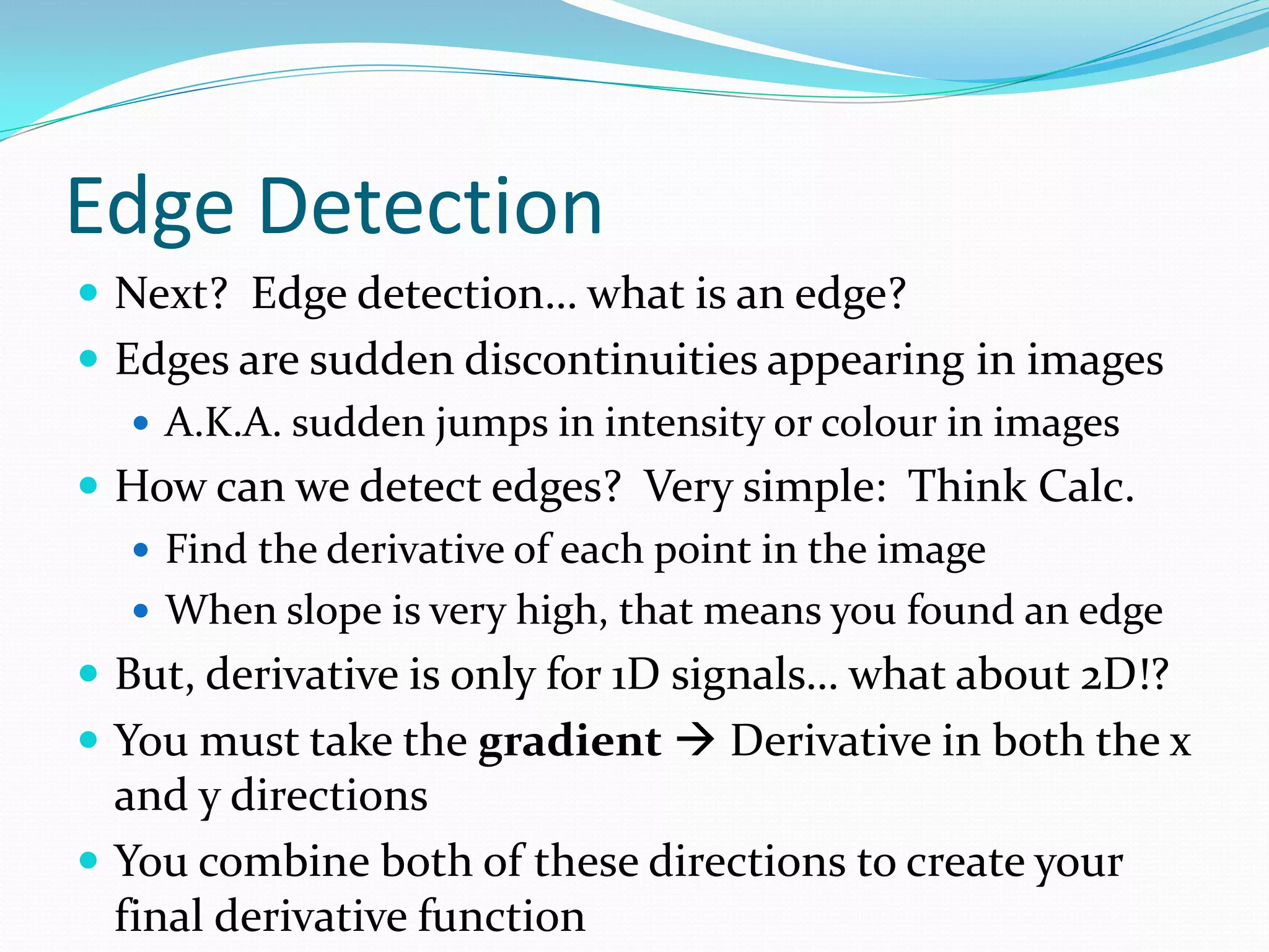
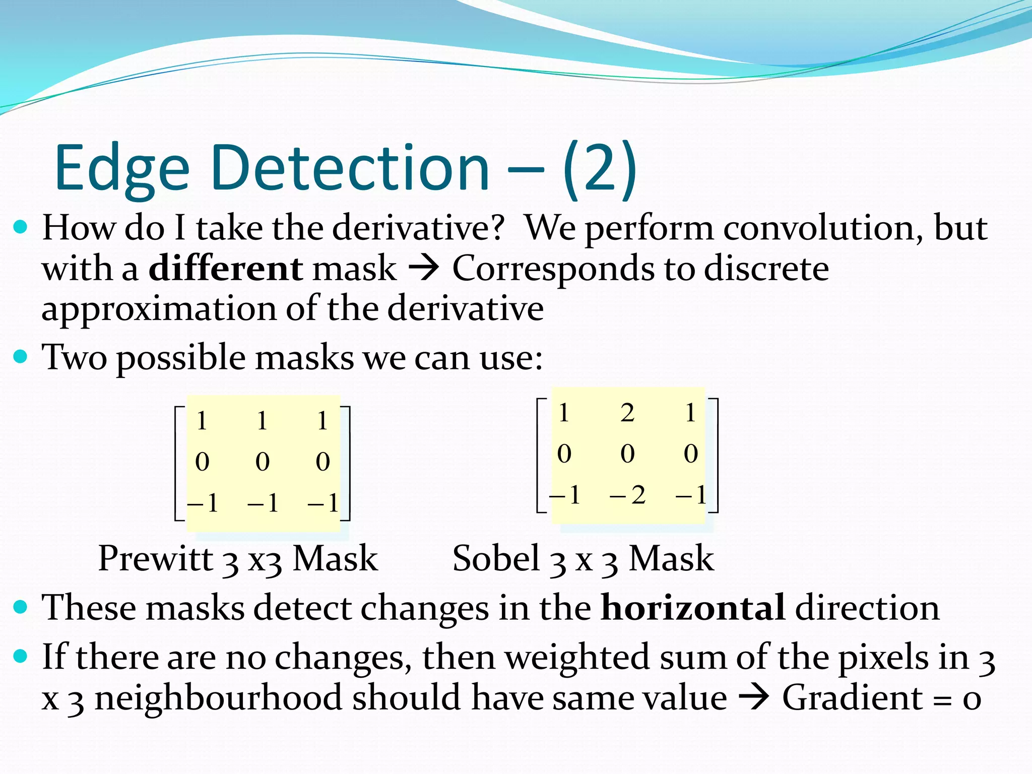
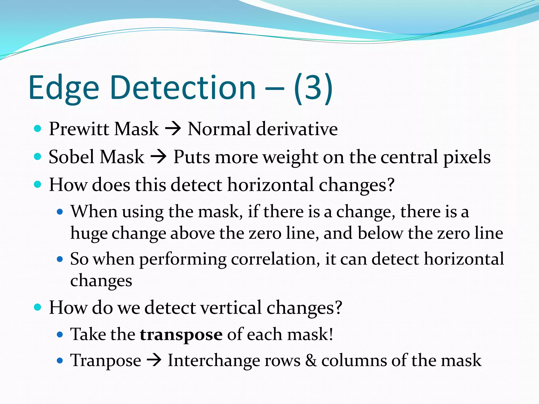
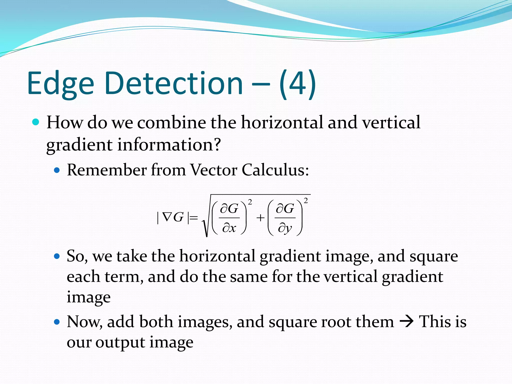
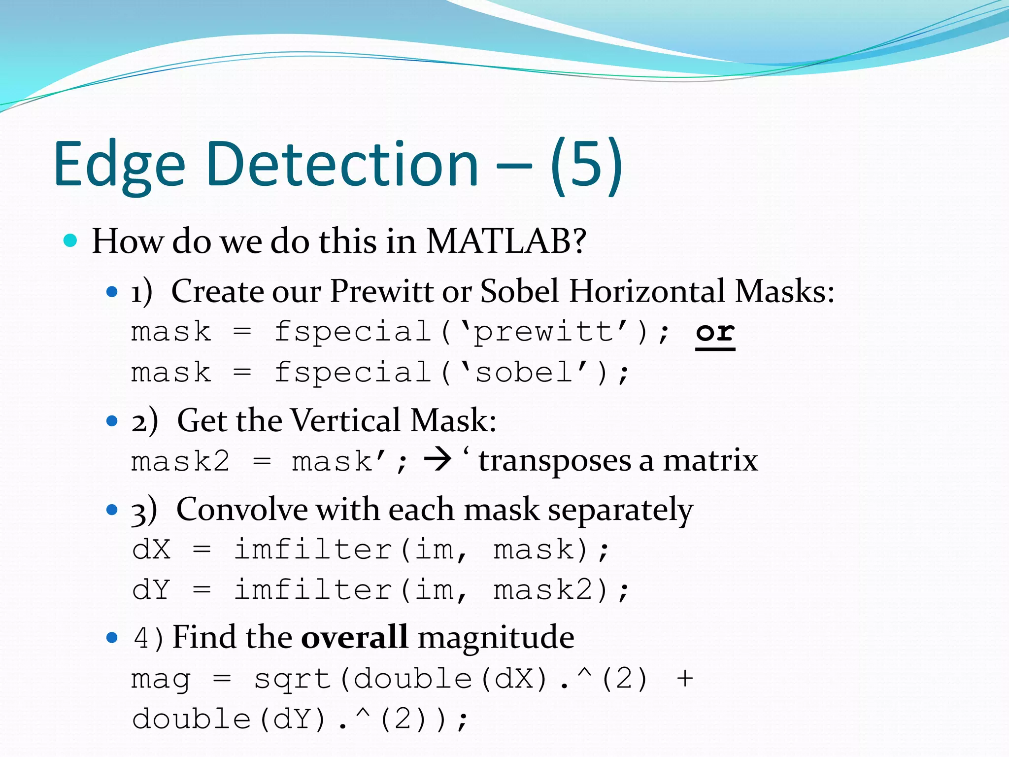
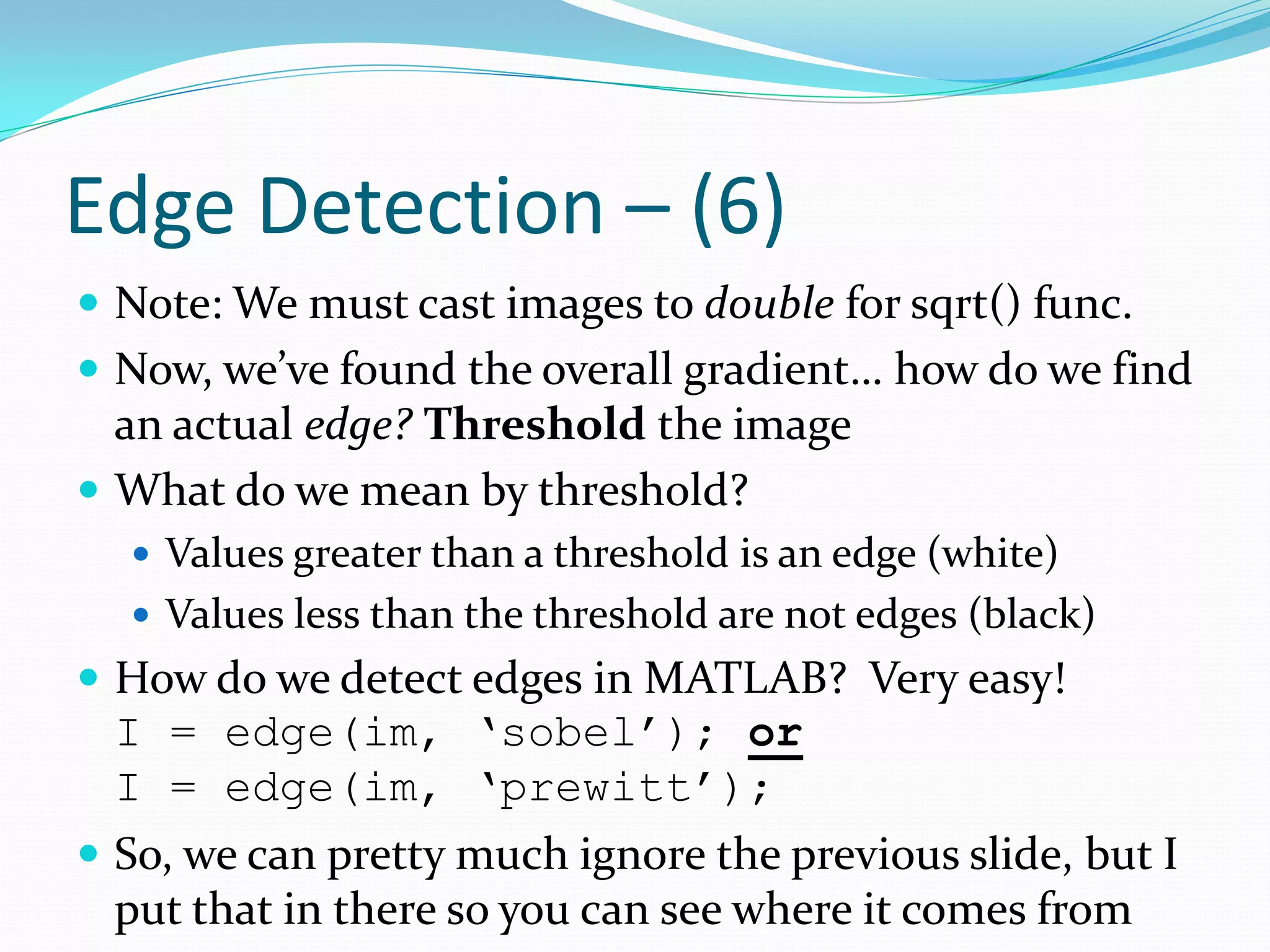
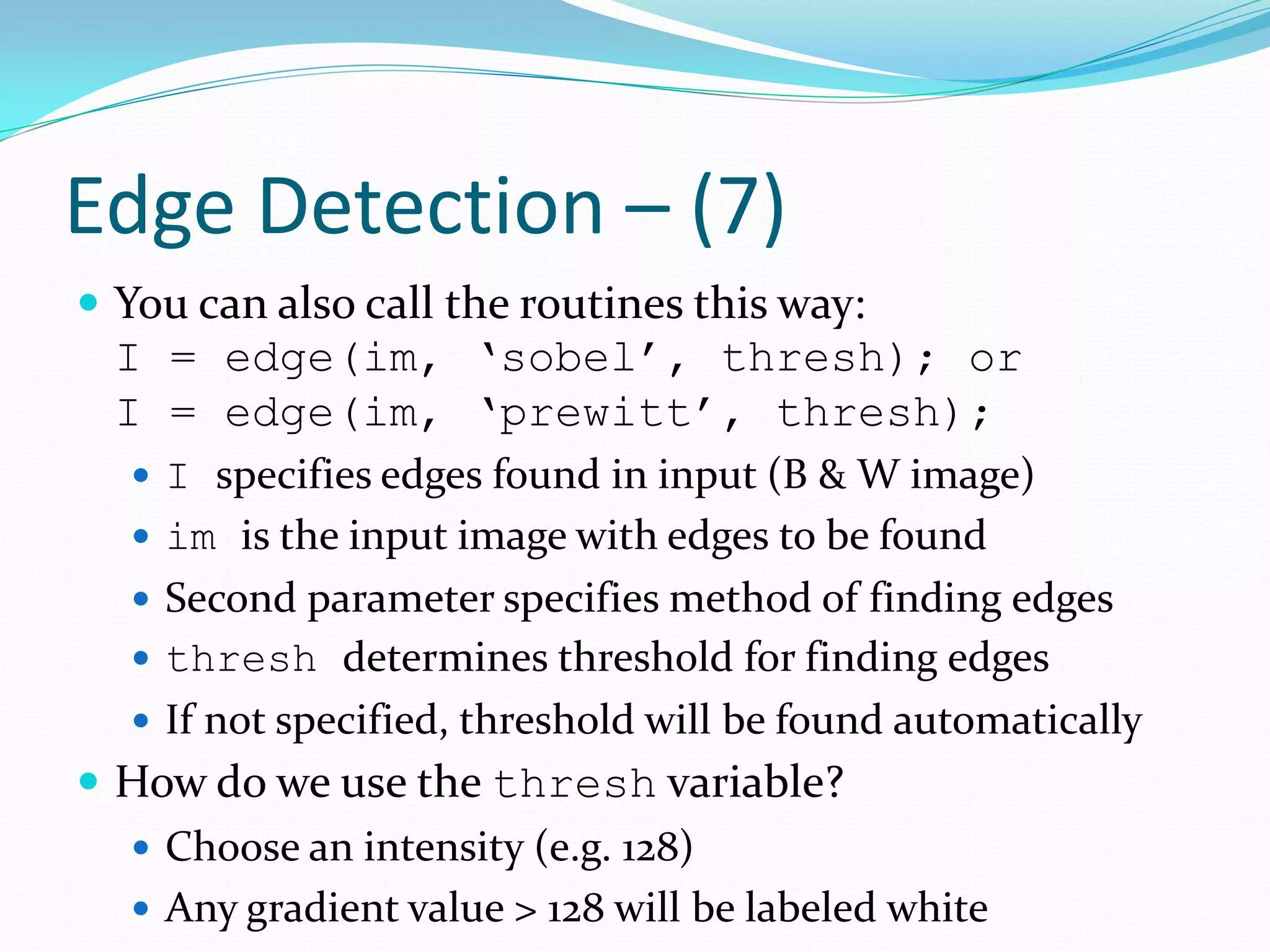
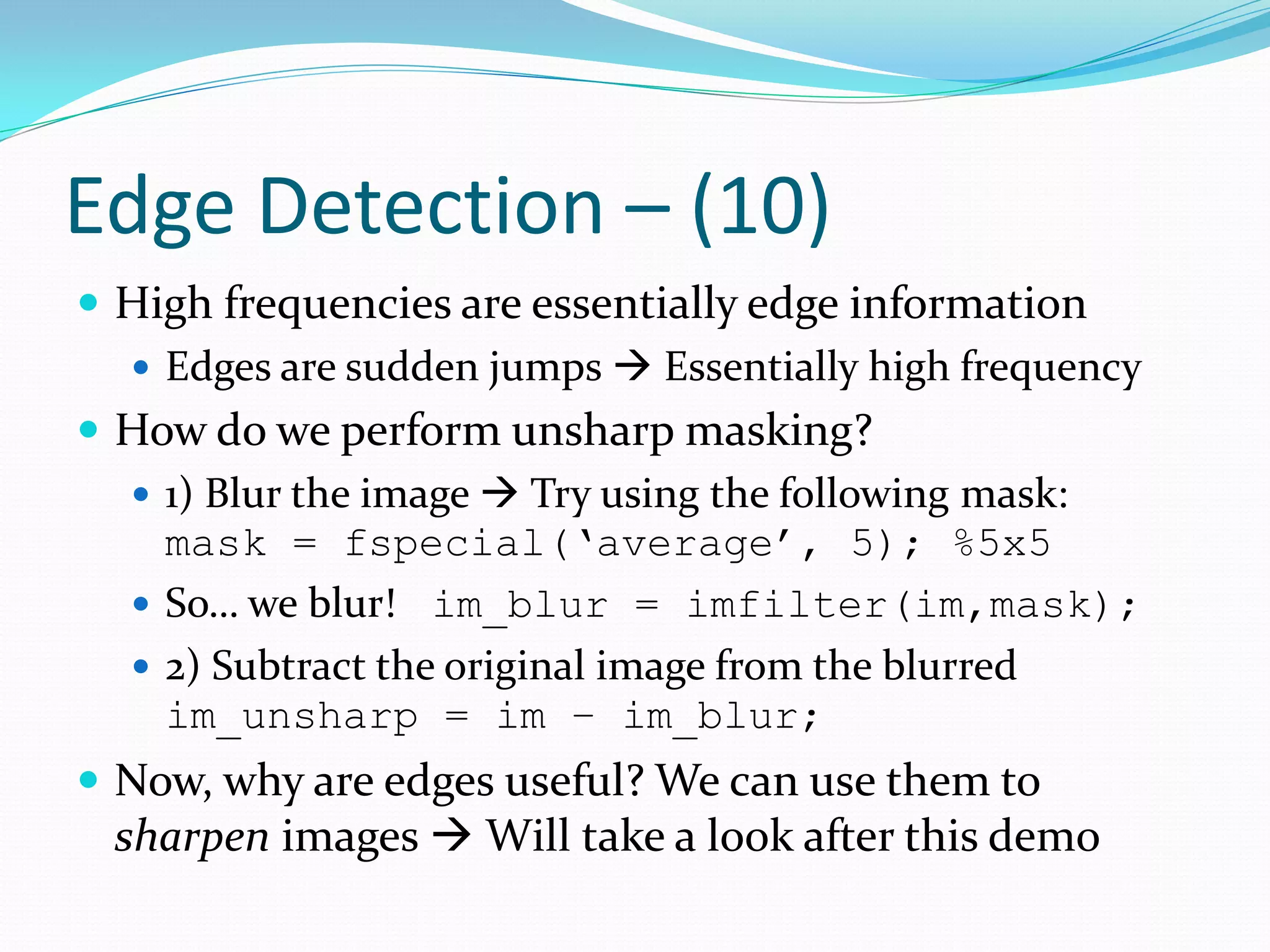
Concepts of edge detection using gradient methods, specific masks, and MATLAB implementation strategies.
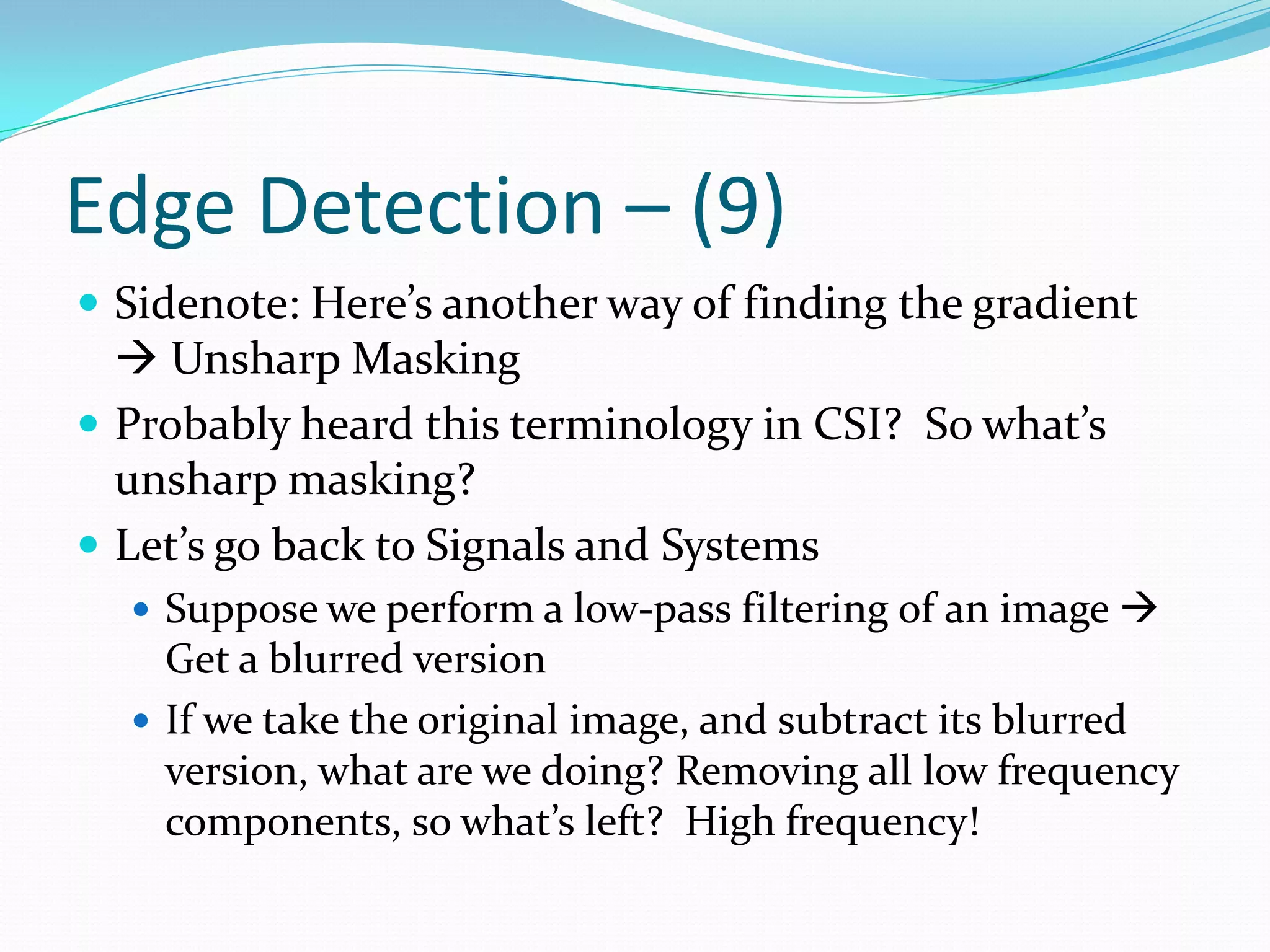
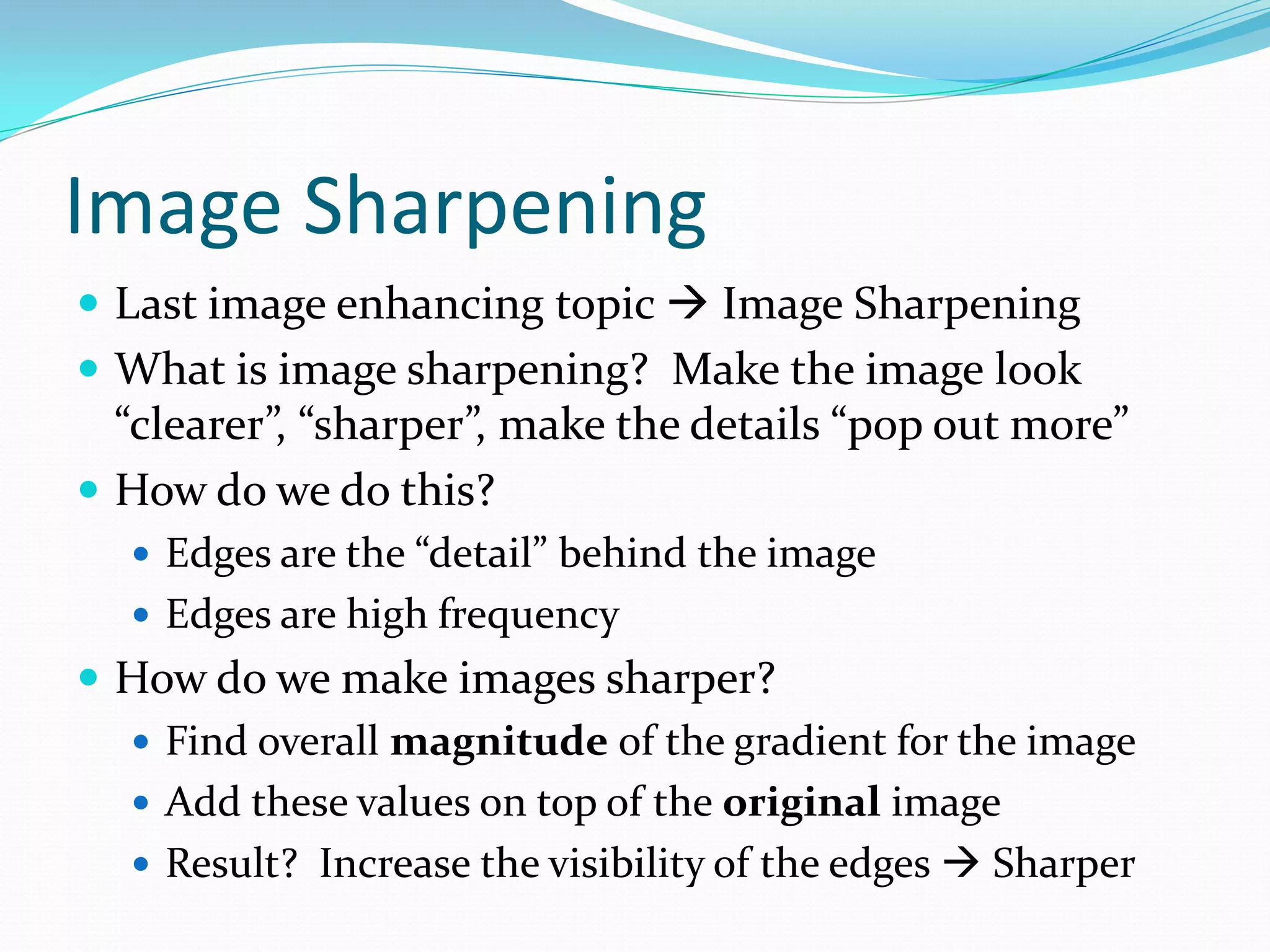
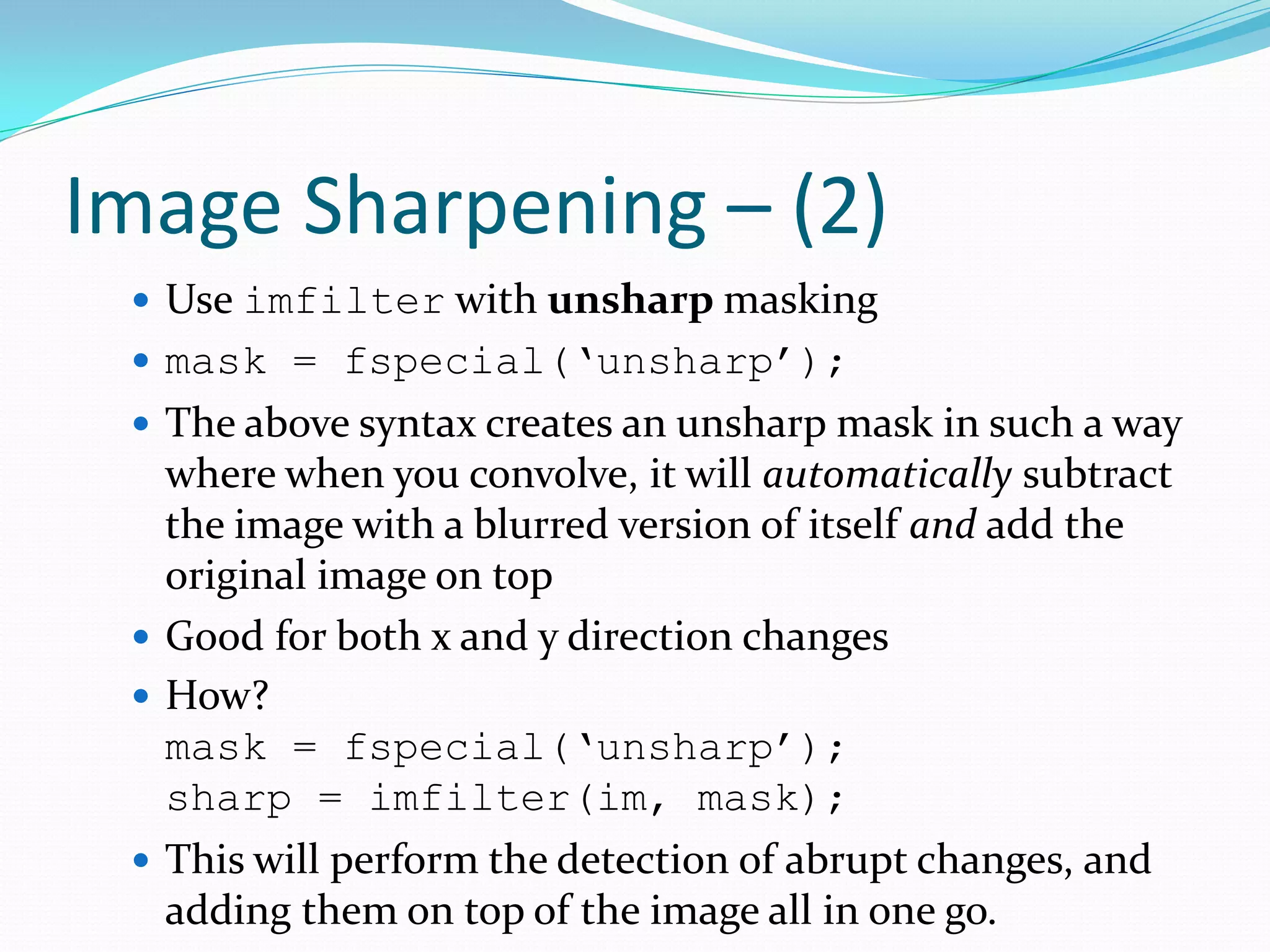
Methods for sharpening images using unsharp masking to enhance details and overall clarity.
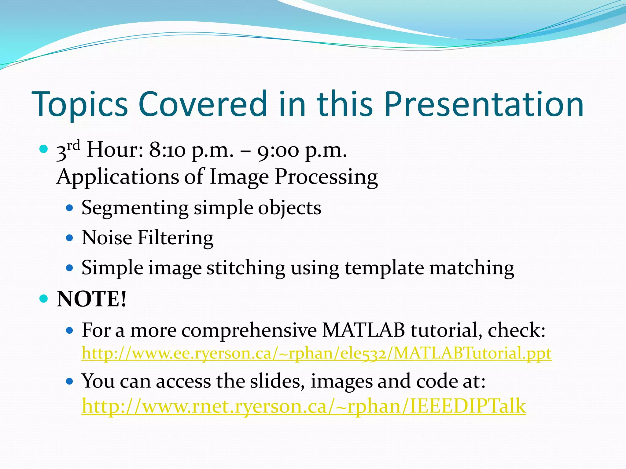
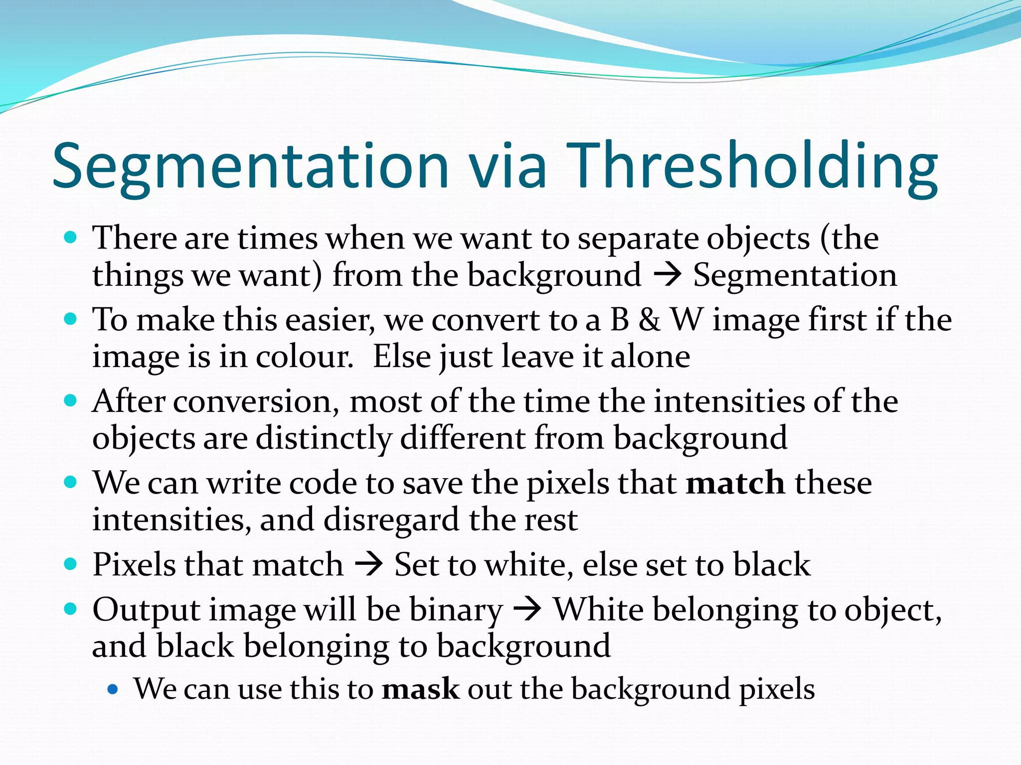
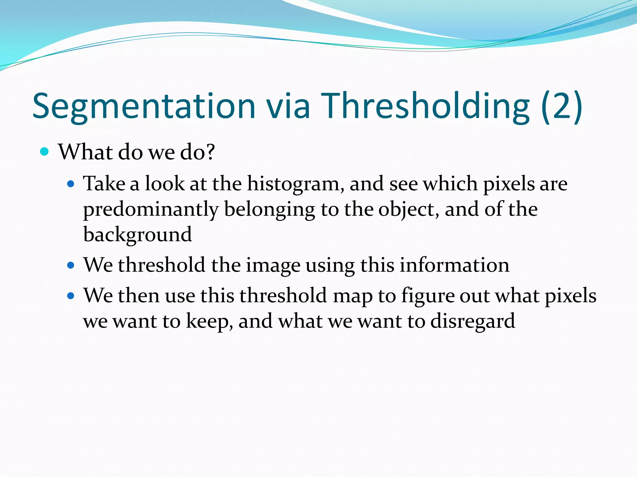
Discussion on application areas of image processing, including segmentation and the methods used.
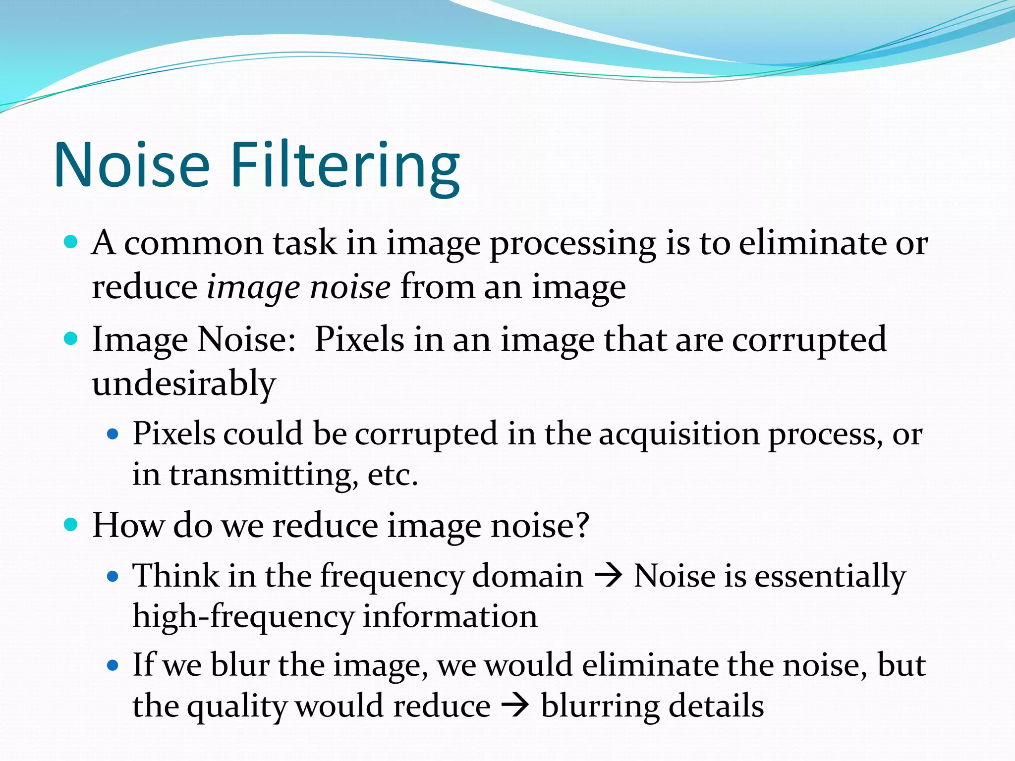
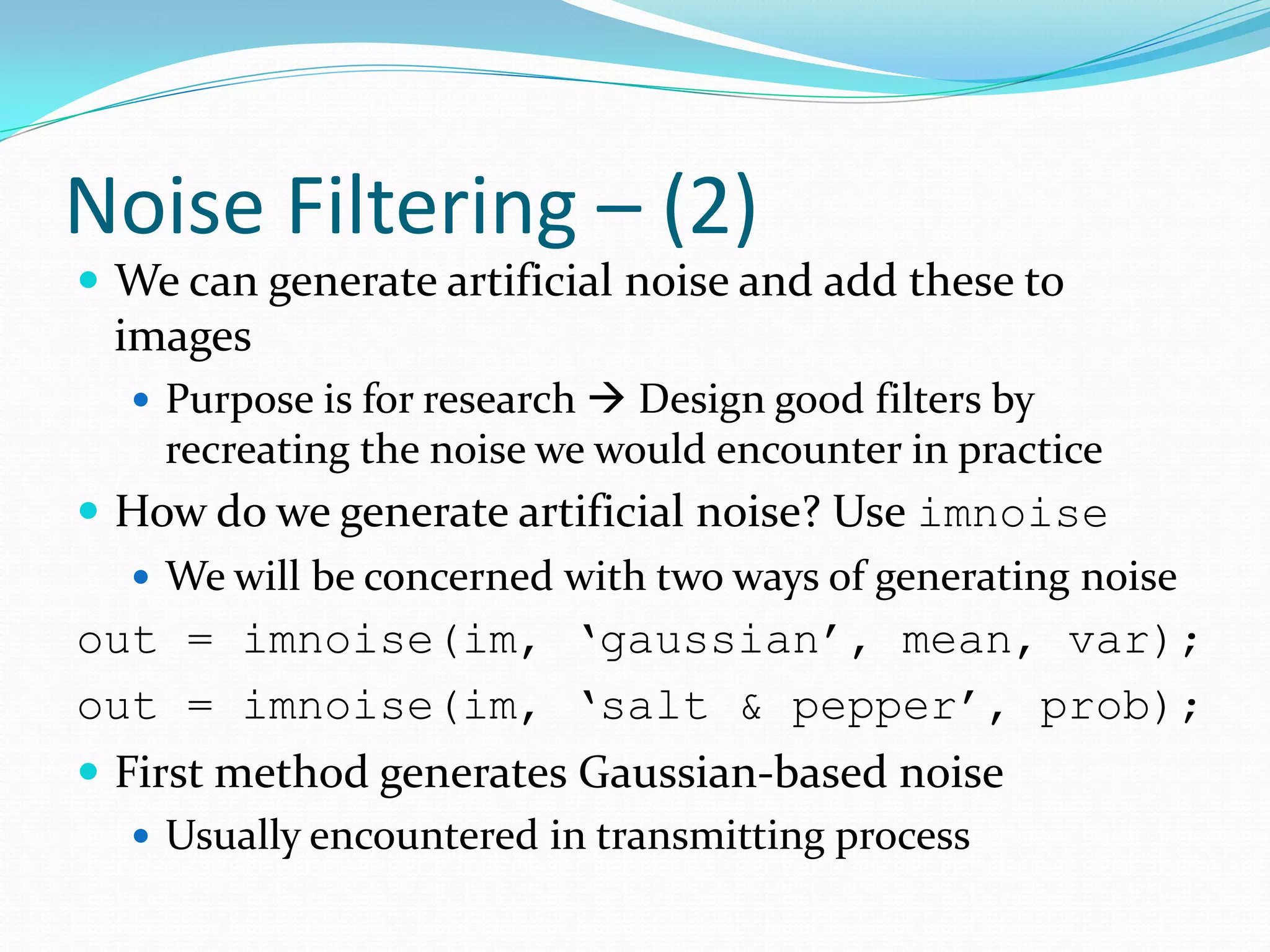
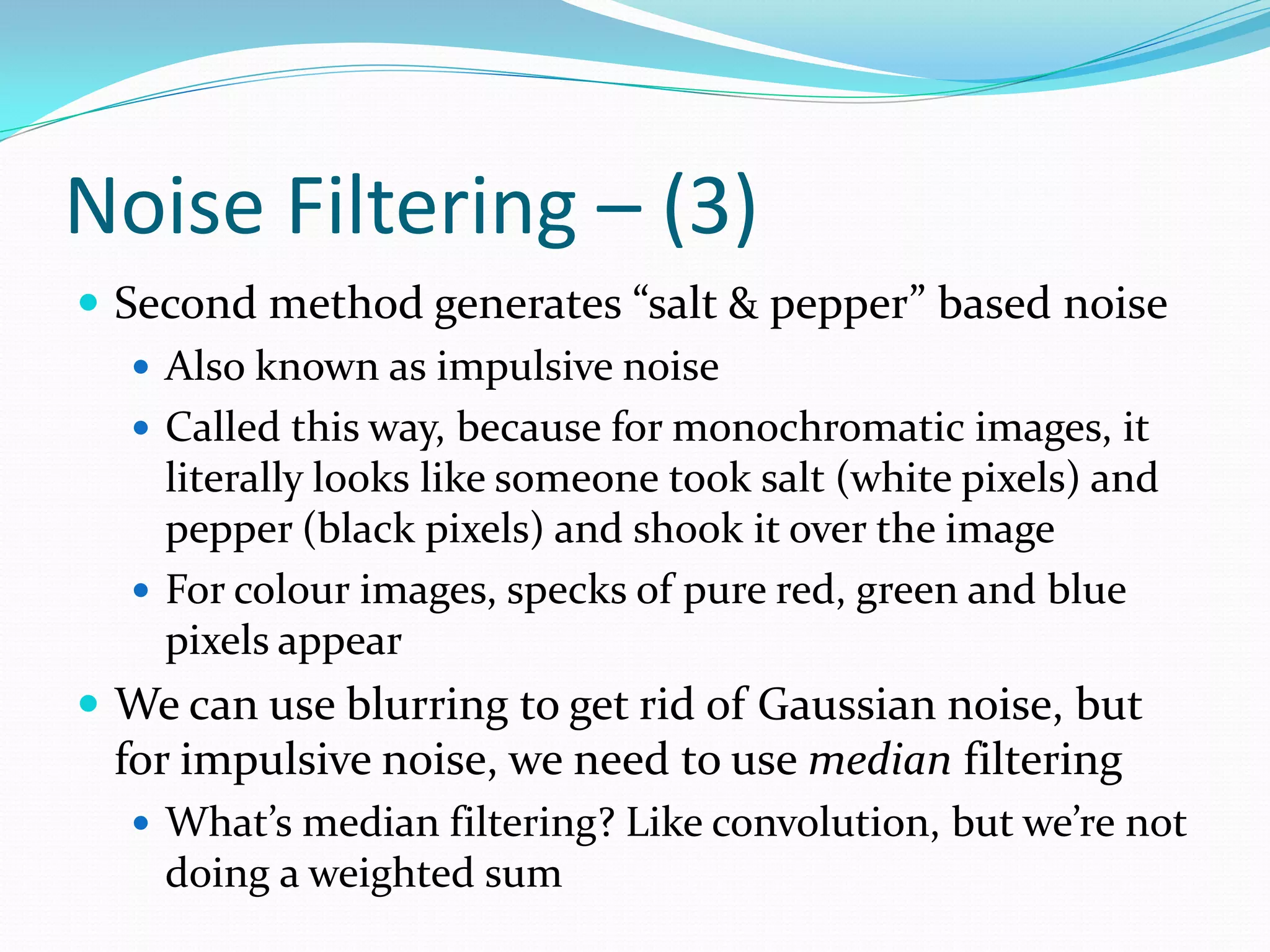
Methods for noise reduction in images, including Gaussian noise and using median filtering.
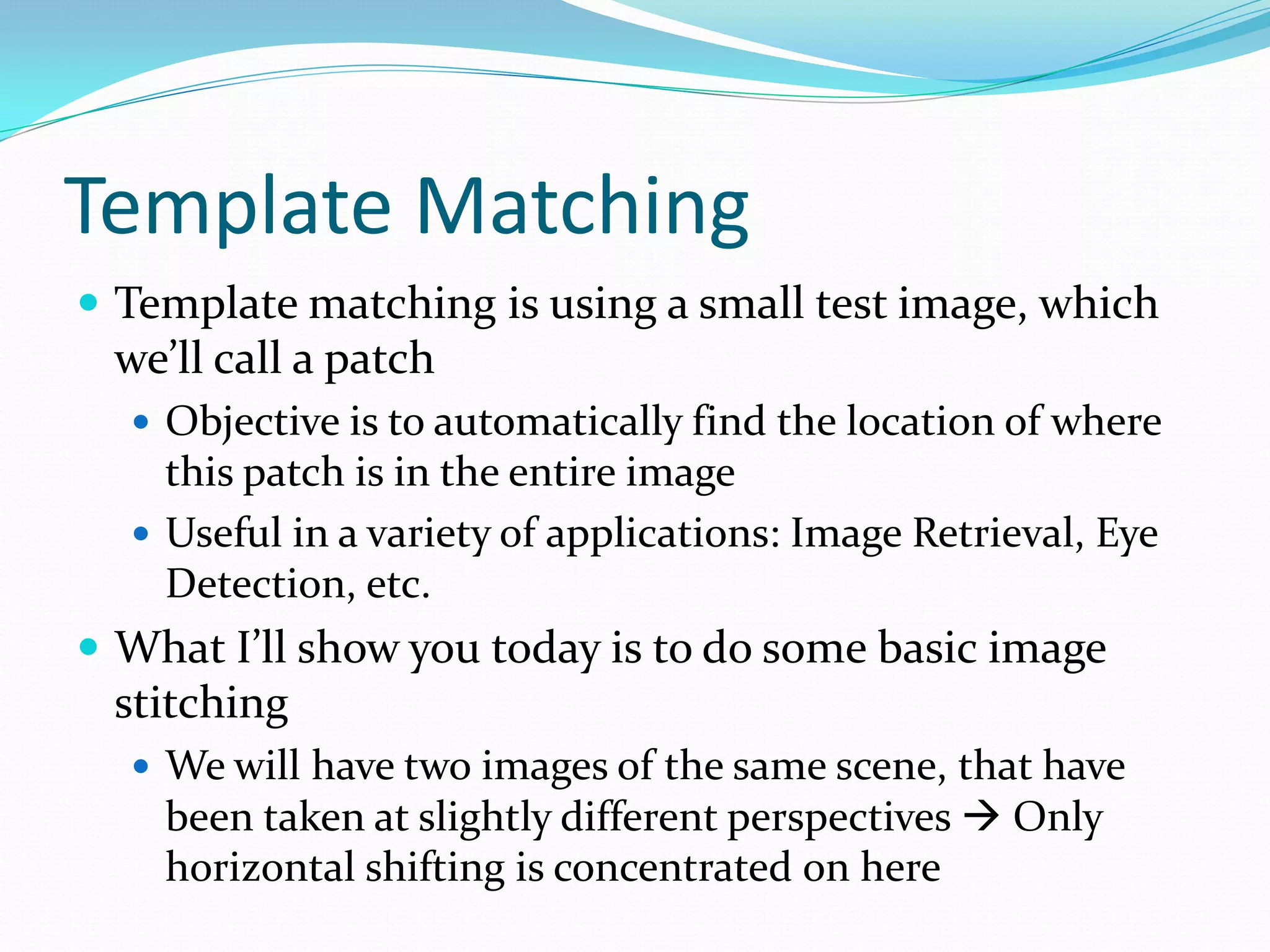
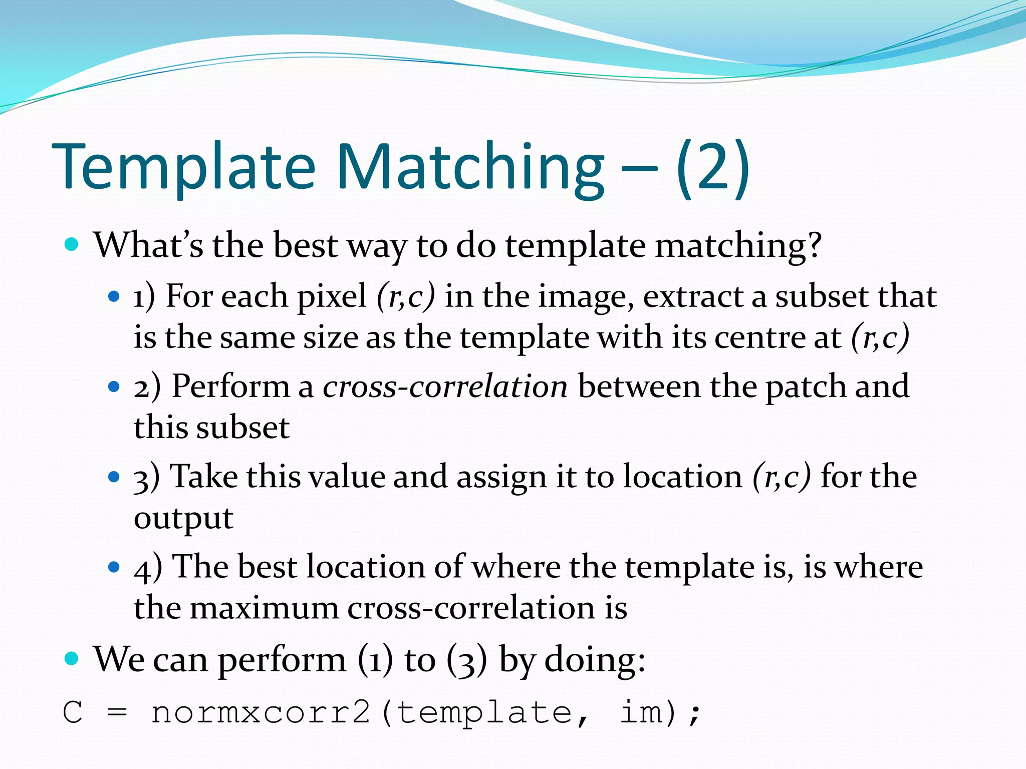
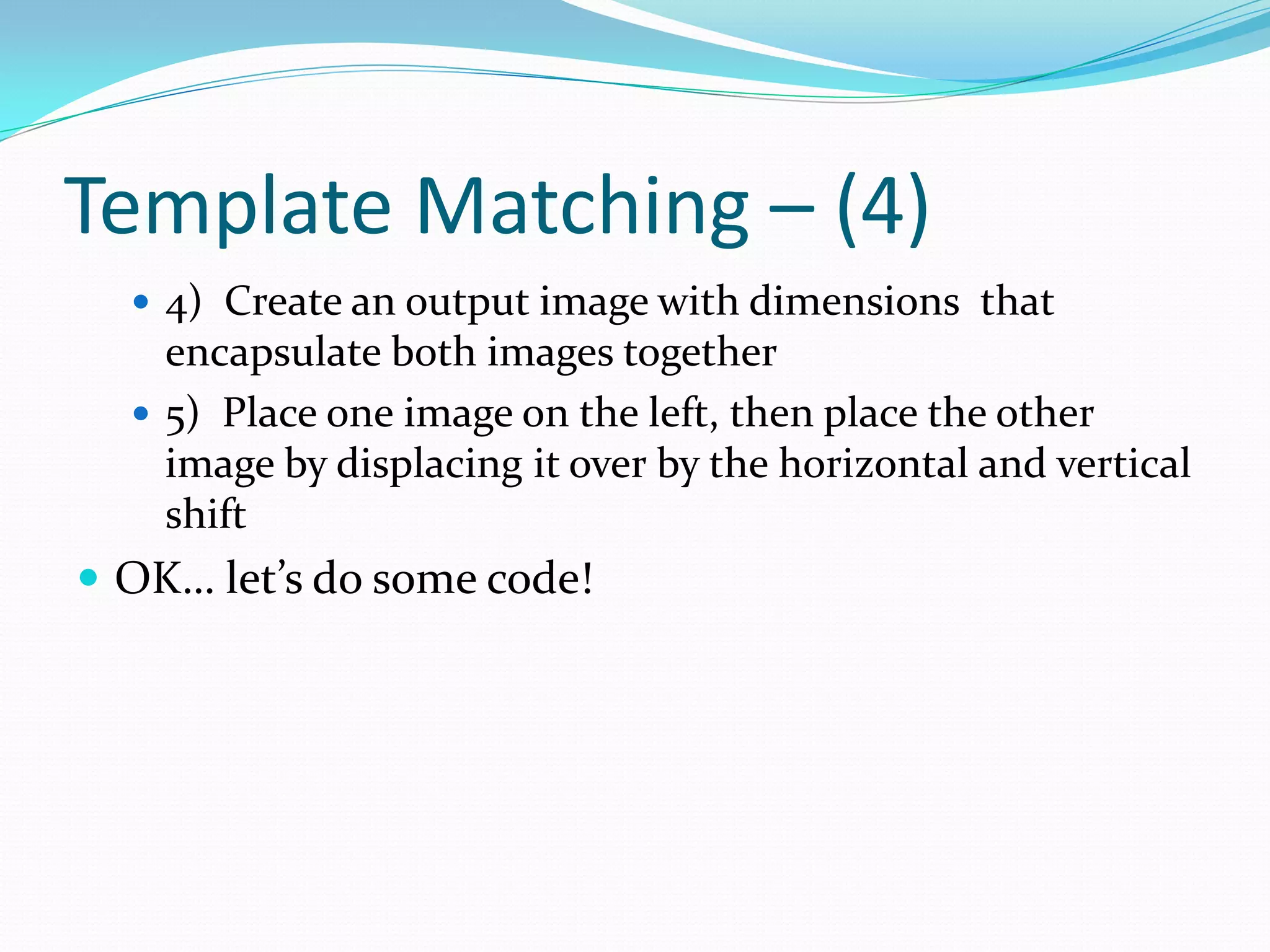
Introduction and methods for template matching to locate patches within images, focusing on image stitching.
Wrap-up of the presentation, highlighting resources for further learning and practical applications of MATLAB in image processing.