Lecture 13 (Usage of Fourier transform in image processing)
This document discusses the Fourier transform and its applications in image processing. It begins by explaining the Fourier transform for 1D and 2D continuous and discrete signals. The Fourier transform converts a signal from the time or space domain to the frequency domain. It then covers properties of the Fourier transform such as separability and translation. The document concludes by mentioning references for further reading on image processing and computer vision topics.
Overview of Fourier Transform applications in signals and image processing. Outlines main topics including continuous and discrete signals, and Fast Fourier Transform.
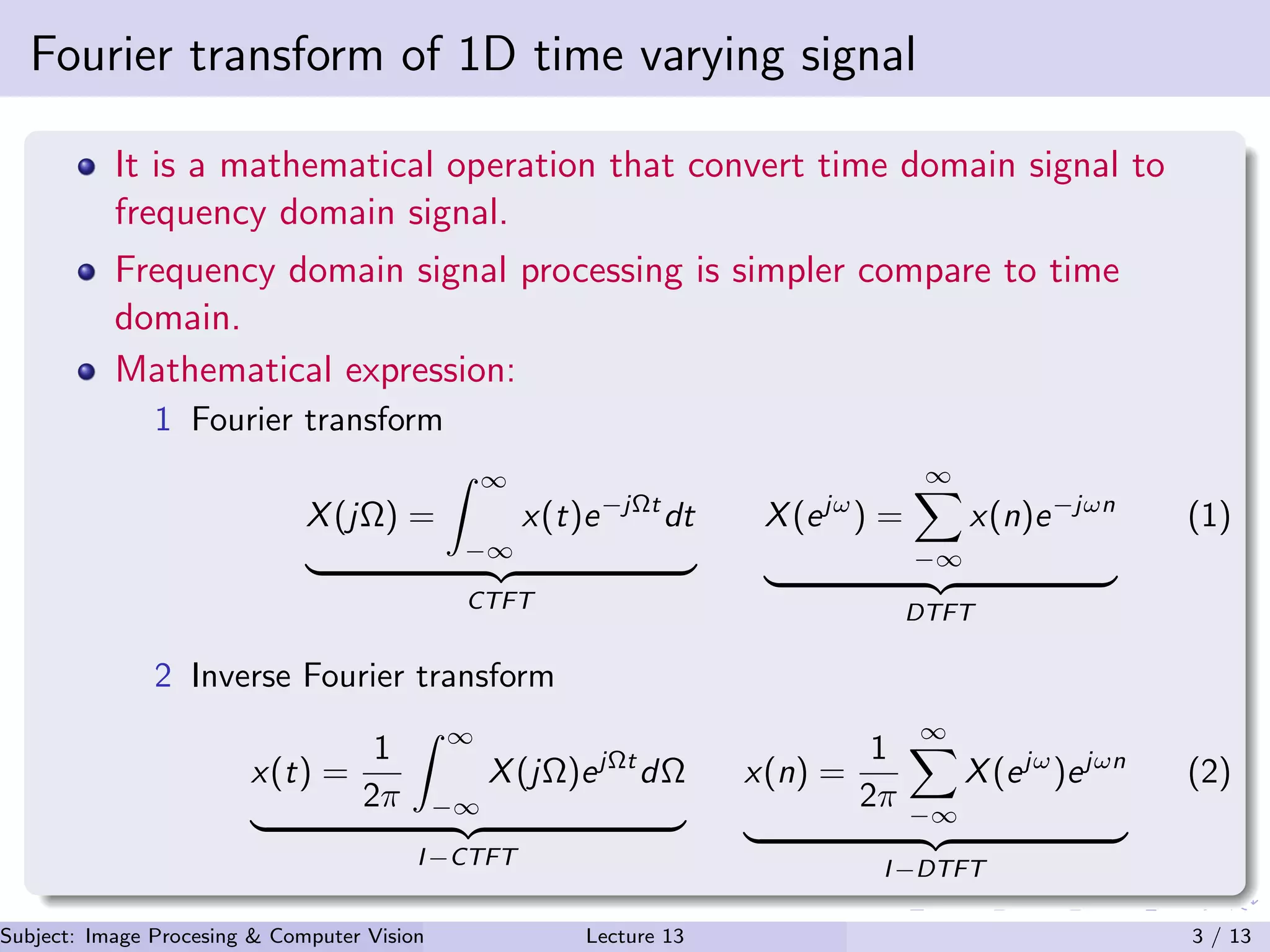
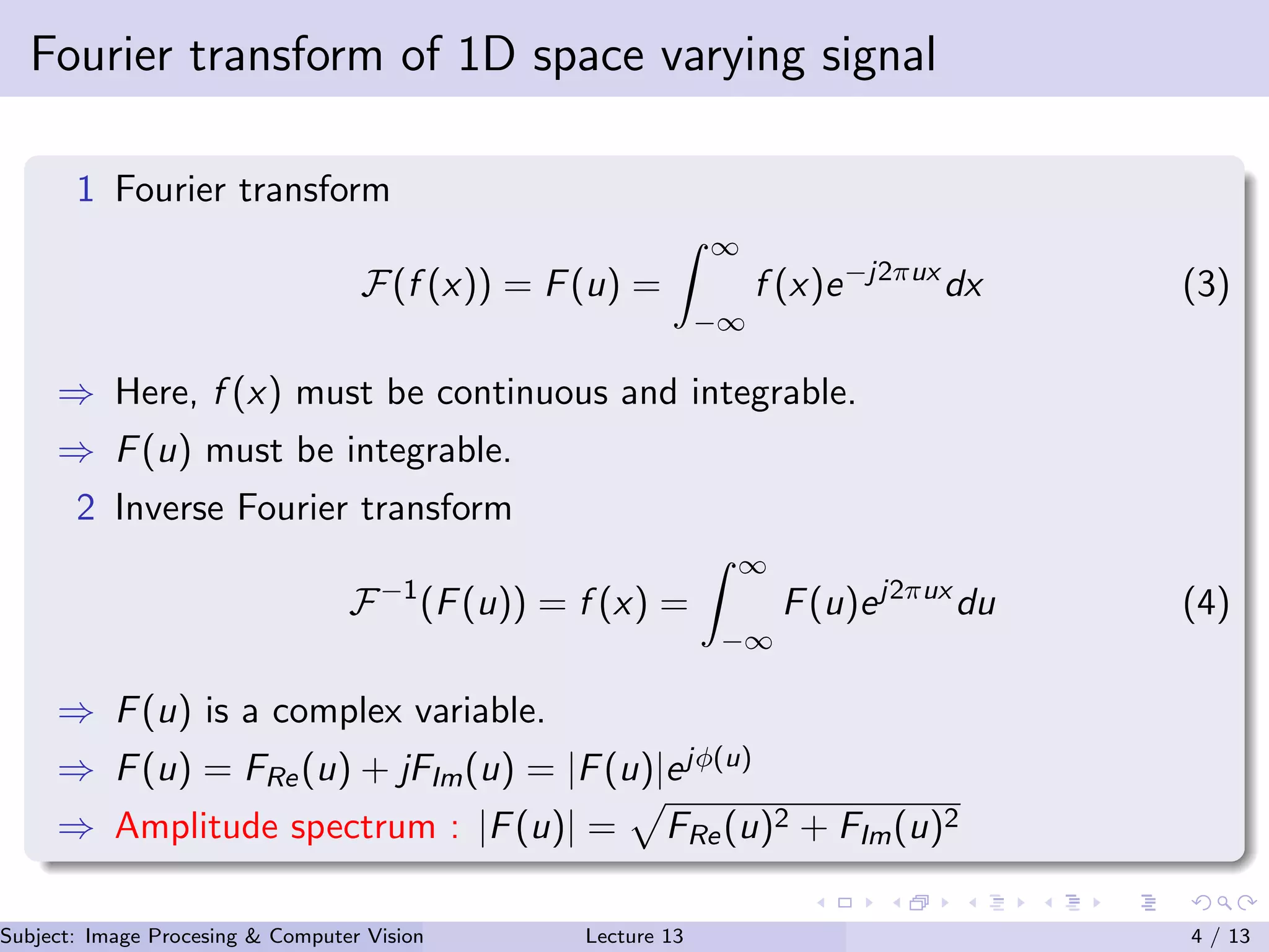
Explains 1D Fourier transform operations and inverses in both time and frequency domains, focusing on mathematical representations for continuous and discrete signals.
Discusses 2D Fourier transforms for image signals, including amplitudes and phases. Explains how to compute the transform and its inverse for 2D signals.
Provides a specific example for computing the Fourier transform of a defined 2D signal, illustrating the amplitude spectrum of the transfer.
Describes DFT and Inverse DFT formulations for 2D signals, including frequency variables for pixel grids. Illustrates the process in square images.
Details properties like separability and translation of Fourier transforms, providing mathematical expressions for DFT and I-DFT transformations.
Lists foundational texts and resources in image processing, computer vision, and detailed DFT applications for additional reading.
Lecture 13 (Usage of Fourier transform in image processing)
1.
Usage of FourierTransform in Image Processing Subject: Image Procesing & Computer Vision Dr. Varun Kumar Subject: Image Procesing & Computer Vision Dr. Varun Kumar (IIIT Surat)Lecture 13 1 / 13
2.
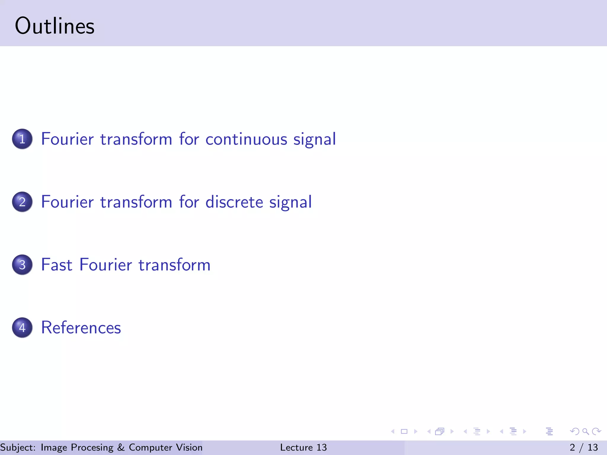
Outlines 1 Fourier transformfor continuous signal 2 Fourier transform for discrete signal 3 Fast Fourier transform 4 References Subject: Image Procesing & Computer Vision Dr. Varun Kumar (IIIT Surat)Lecture 13 2 / 13
3.
Fourier transform of1D time varying signal It is a mathematical operation that convert time domain signal to frequency domain signal. Frequency domain signal processing is simpler compare to time domain. Mathematical expression: 1 Fourier transform X(jΩ) = ∞ −∞ x(t)e−jΩt dt CTFT X(ejω ) = ∞ −∞ x(n)e−jωn DTFT (1) 2 Inverse Fourier transform x(t) = 1 2π ∞ −∞ X(jΩ)ejΩt dΩ I−CTFT x(n) = 1 2π ∞ −∞ X(ejω )ejωn I−DTFT (2) Subject: Image Procesing & Computer Vision Dr. Varun Kumar (IIIT Surat)Lecture 13 3 / 13
4.
Fourier transform of1D space varying signal 1 Fourier transform F(f (x)) = F(u) = ∞ −∞ f (x)e−j2πux dx (3) ⇒ Here, f (x) must be continuous and integrable. ⇒ F(u) must be integrable. 2 Inverse Fourier transform F−1 (F(u)) = f (x) = ∞ −∞ F(u)ej2πux du (4) ⇒ F(u) is a complex variable. ⇒ F(u) = FRe(u) + jFIm(u) = |F(u)|ejφ(u) ⇒ Amplitude spectrum : |F(u)| = FRe(u)2 + FIm(u)2 Subject: Image Procesing & Computer Vision Dr. Varun Kumar (IIIT Surat)Lecture 13 4 / 13
5.
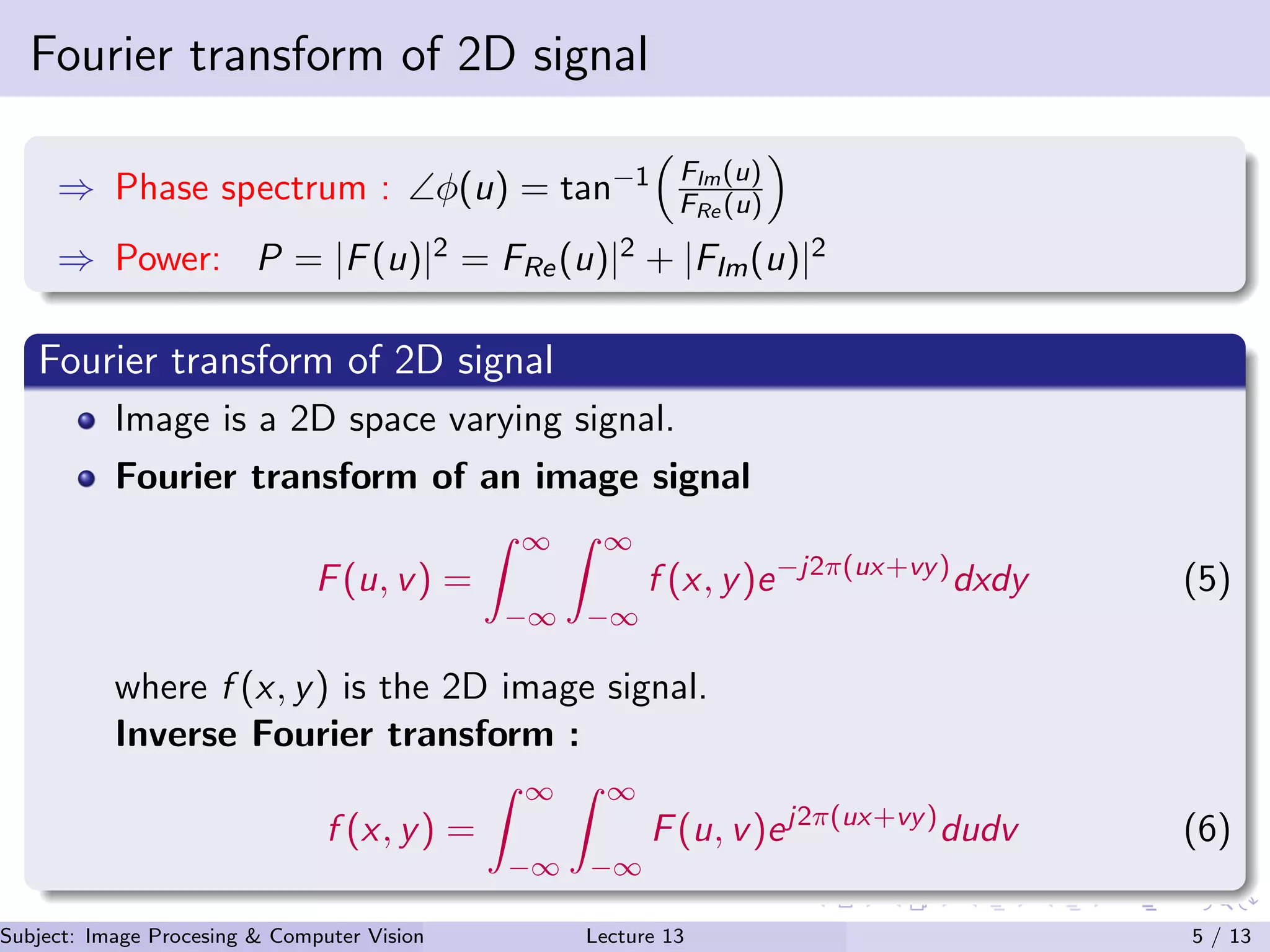
Fourier transform of2D signal ⇒ Phase spectrum : ∠φ(u) = tan−1 FIm(u) FRe (u) ⇒ Power: P = |F(u)|2 = FRe(u)|2 + |FIm(u)|2 Fourier transform of 2D signal Image is a 2D space varying signal. Fourier transform of an image signal F(u, v) = ∞ −∞ ∞ −∞ f (x, y)e−j2π(ux+vy) dxdy (5) where f (x, y) is the 2D image signal. Inverse Fourier transform : f (x, y) = ∞ −∞ ∞ −∞ F(u, v)ej2π(ux+vy) dudv (6) Subject: Image Procesing & Computer Vision Dr. Varun Kumar (IIIT Surat)Lecture 13 5 / 13
6.
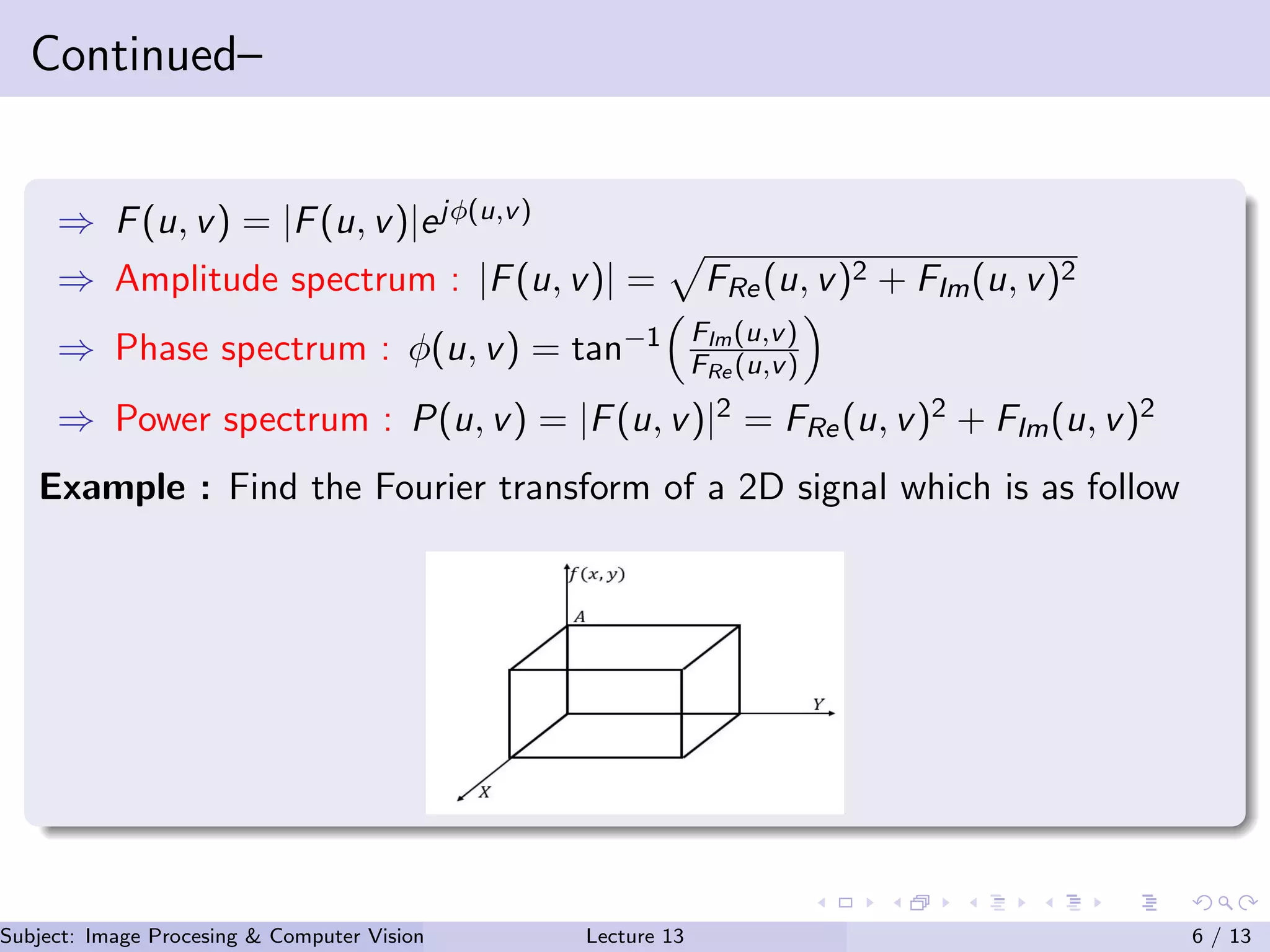
Continued– ⇒ F(u, v)= |F(u, v)|ejφ(u,v) ⇒ Amplitude spectrum : |F(u, v)| = FRe(u, v)2 + FIm(u, v)2 ⇒ Phase spectrum : φ(u, v) = tan−1 FIm(u,v) FRe (u,v) ⇒ Power spectrum : P(u, v) = |F(u, v)|2 = FRe(u, v)2 + FIm(u, v)2 Example : Find the Fourier transform of a 2D signal which is as follow Subject: Image Procesing & Computer Vision Dr. Varun Kumar (IIIT Surat)Lecture 13 6 / 13
7.
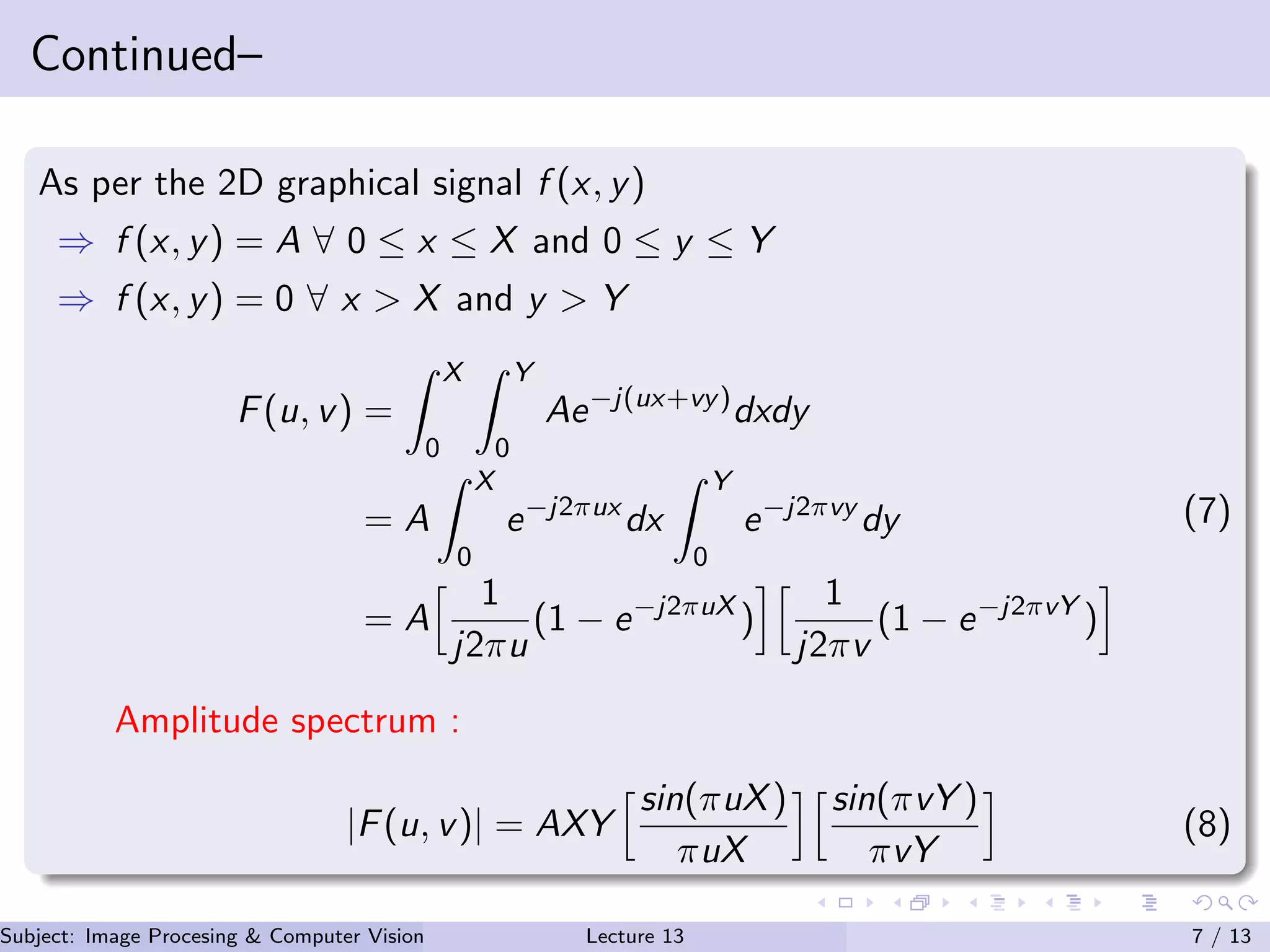
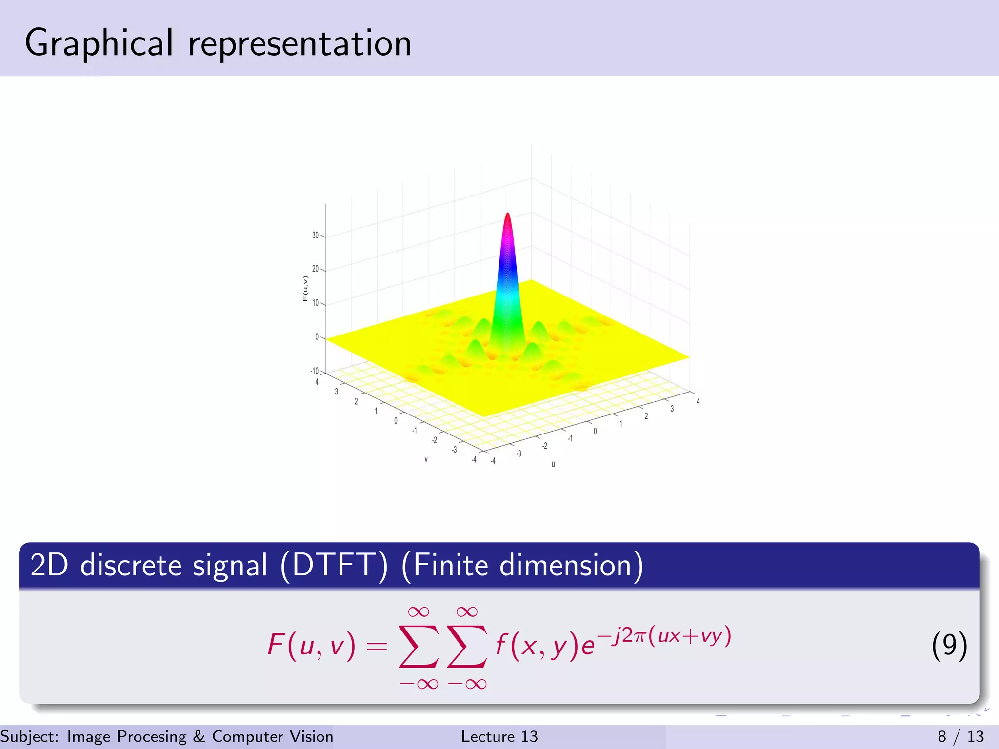
Continued– As per the2D graphical signal f (x, y) ⇒ f (x, y) = A ∀ 0 ≤ x ≤ X and 0 ≤ y ≤ Y ⇒ f (x, y) = 0 ∀ x > X and y > Y F(u, v) = X 0 Y 0 Ae−j(ux+vy) dxdy = A X 0 e−j2πux dx Y 0 e−j2πvy dy = A 1 j2πu (1 − e−j2πuX ) 1 j2πv (1 − e−j2πvY ) (7) Amplitude spectrum : |F(u, v)| = AXY sin(πuX) πuX sin(πvY ) πvY (8) Subject: Image Procesing & Computer Vision Dr. Varun Kumar (IIIT Surat)Lecture 13 7 / 13
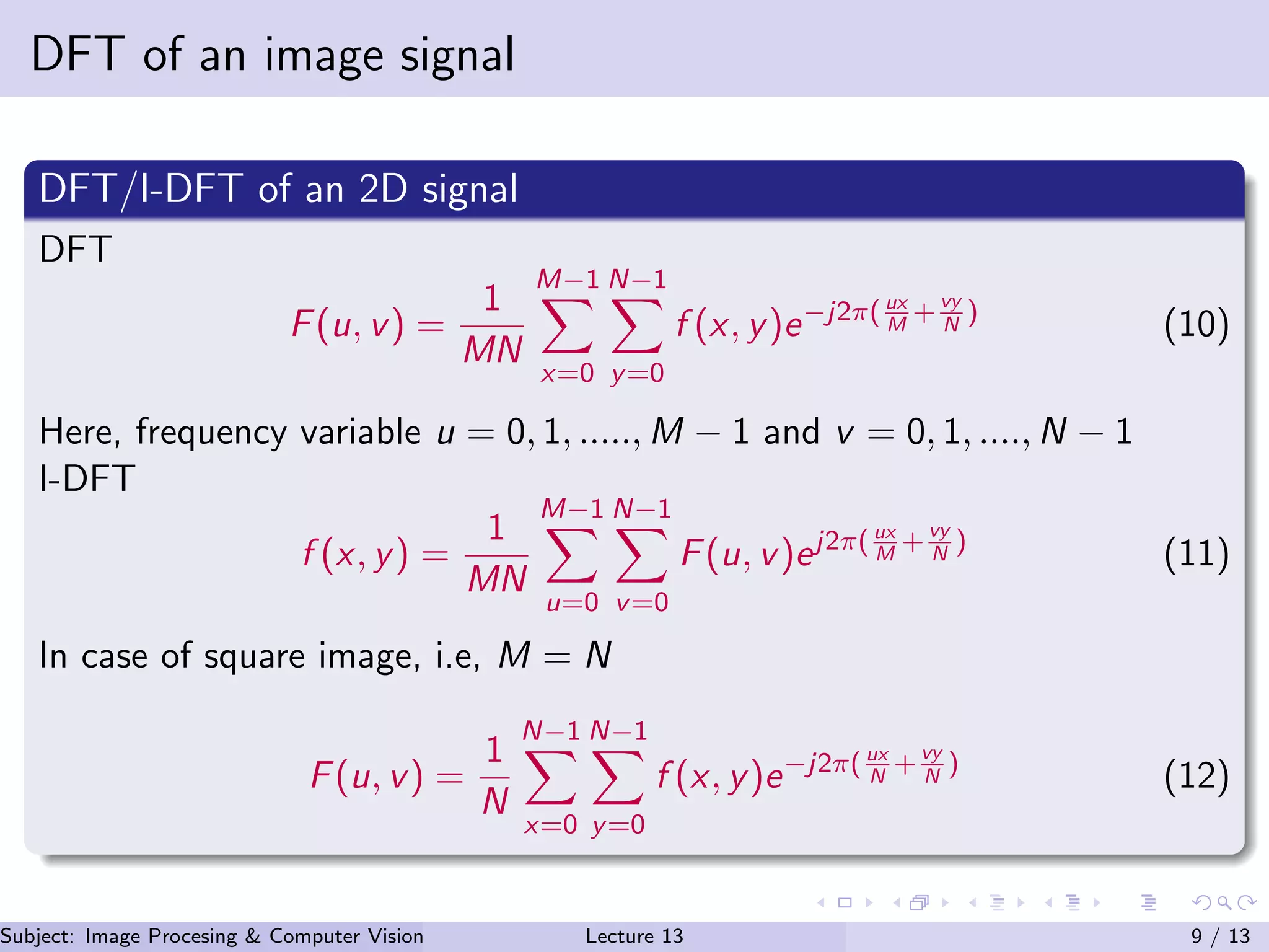
DFT of animage signal DFT/I-DFT of an 2D signal DFT F(u, v) = 1 MN M−1 x=0 N−1 y=0 f (x, y)e−j2π( ux M +vy N ) (10) Here, frequency variable u = 0, 1, ....., M − 1 and v = 0, 1, ...., N − 1 I-DFT f (x, y) = 1 MN M−1 u=0 N−1 v=0 F(u, v)ej2π( ux M +vy N ) (11) In case of square image, i.e, M = N F(u, v) = 1 N N−1 x=0 N−1 y=0 f (x, y)e−j2π( ux N +vy N ) (12) Subject: Image Procesing & Computer Vision Dr. Varun Kumar (IIIT Surat)Lecture 13 9 / 13
10.
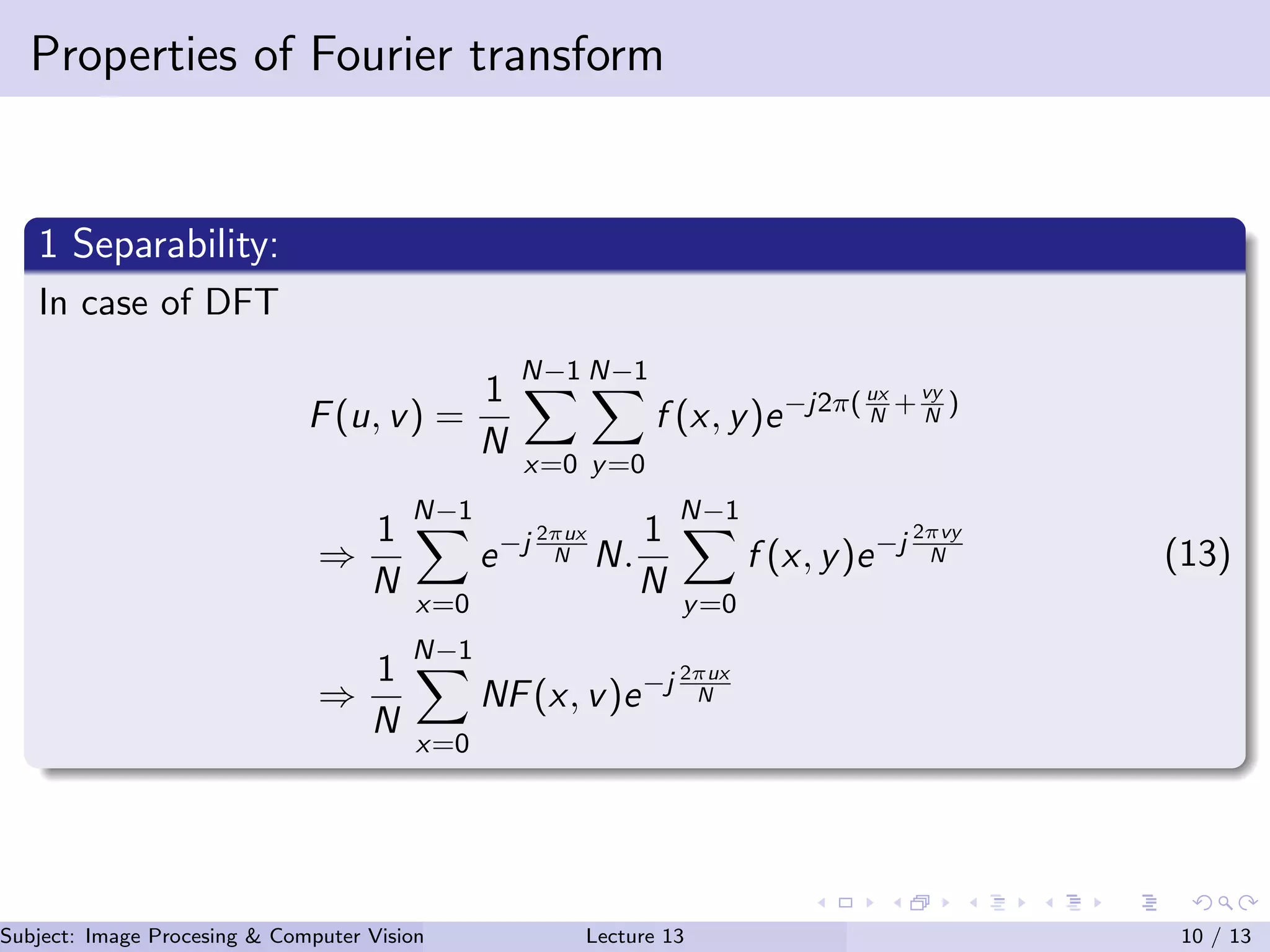
Properties of Fouriertransform 1 Separability: In case of DFT F(u, v) = 1 N N−1 x=0 N−1 y=0 f (x, y)e−j2π(ux N +vy N ) ⇒ 1 N N−1 x=0 e−j 2πux N N. 1 N N−1 y=0 f (x, y)e−j 2πvy N ⇒ 1 N N−1 x=0 NF(x, v)e−j 2πux N (13) Subject: Image Procesing & Computer Vision Dr. Varun Kumar (IIIT Surat)Lecture 13 10 / 13
11.
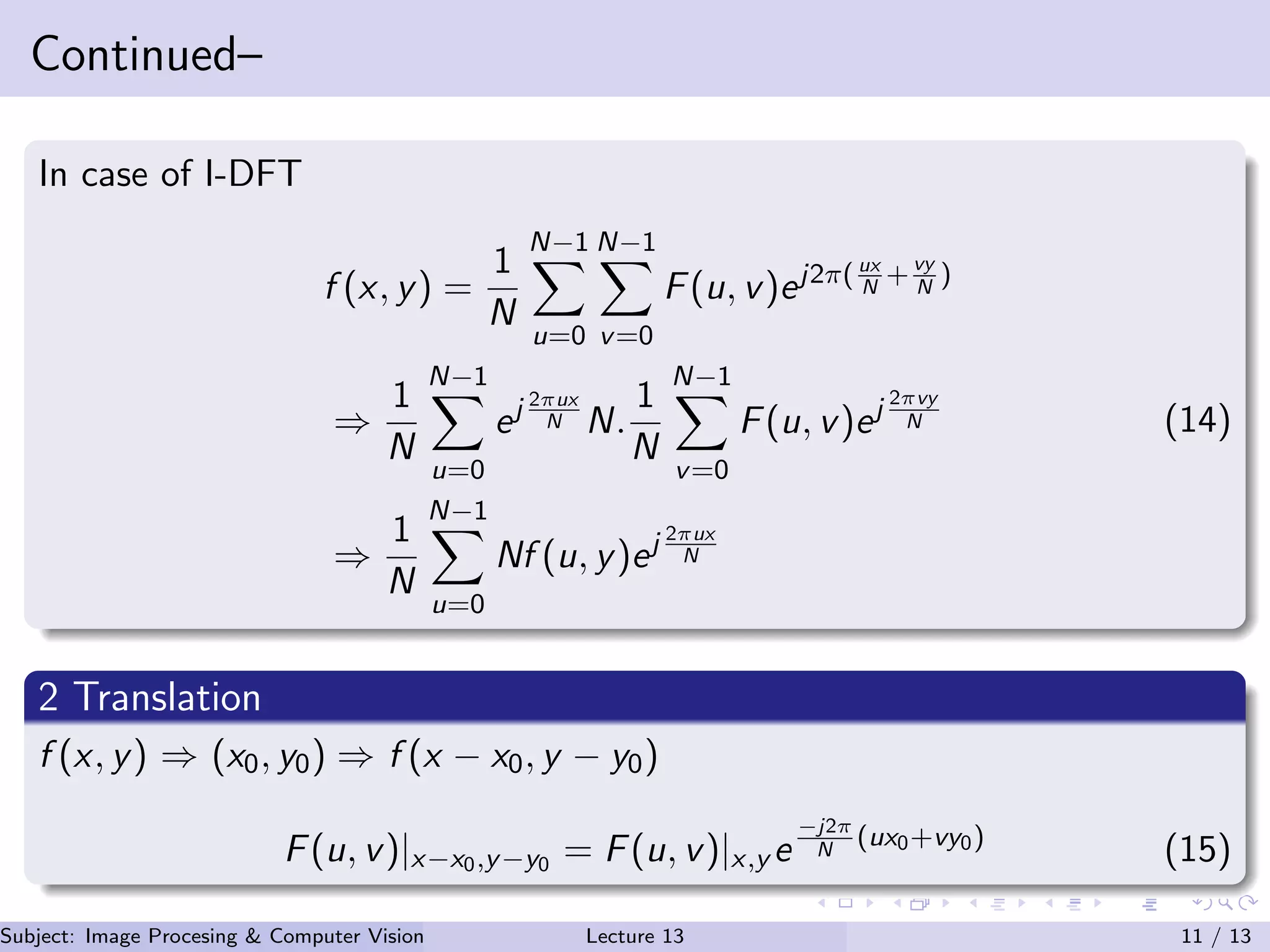
Continued– In case ofI-DFT f (x, y) = 1 N N−1 u=0 N−1 v=0 F(u, v)ej2π( ux N +vy N ) ⇒ 1 N N−1 u=0 ej 2πux N N. 1 N N−1 v=0 F(u, v)ej 2πvy N ⇒ 1 N N−1 u=0 Nf (u, y)ej 2πux N (14) 2 Translation f (x, y) ⇒ (x0, y0) ⇒ f (x − x0, y − y0) F(u, v)|x−x0,y−y0 = F(u, v)|x,y e −j2π N (ux0+vy0) (15) Subject: Image Procesing & Computer Vision Dr. Varun Kumar (IIIT Surat)Lecture 13 11 / 13
12.
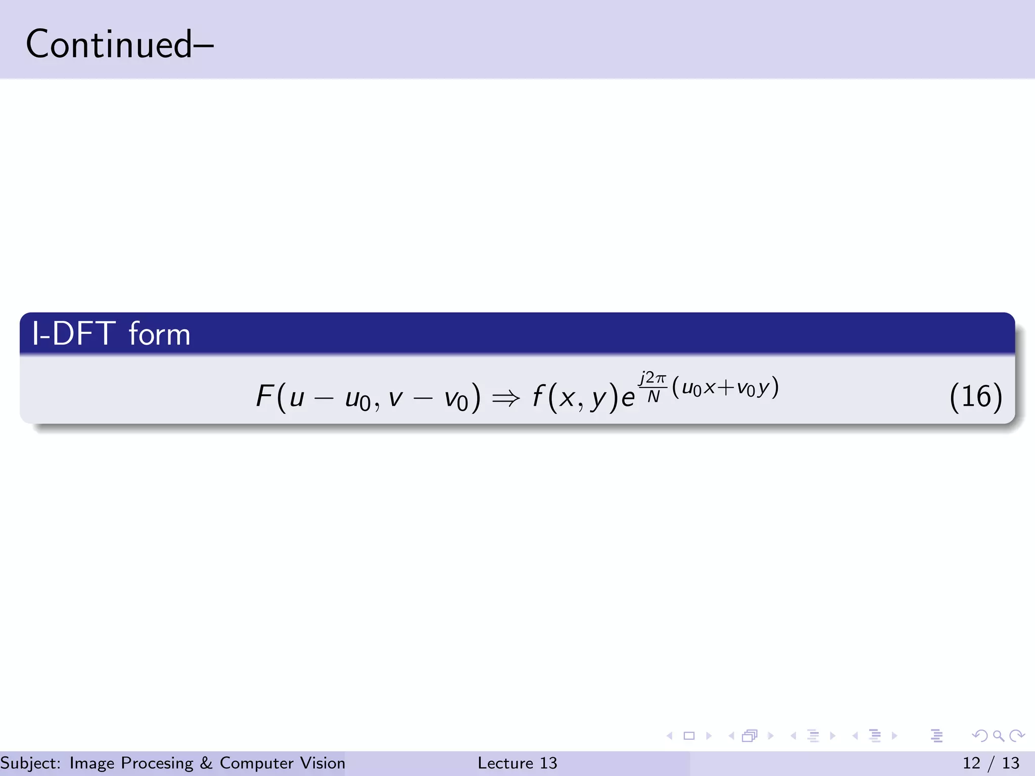
Continued– I-DFT form F(u −u0, v − v0) ⇒ f (x, y)e j2π N (u0x+v0y) (16) Subject: Image Procesing & Computer Vision Dr. Varun Kumar (IIIT Surat)Lecture 13 12 / 13
13.
References M. Sonka, V.Hlavac, and R. Boyle, Image processing, analysis, and machine vision. Cengage Learning, 2014. D. A. Forsyth and J. Ponce, “A modern approach,” Computer vision: a modern approach, vol. 17, pp. 21–48, 2003. L. Shapiro and G. Stockman, “Computer vision prentice hall,” Inc., New Jersey, 2001. R. C. Gonzalez, R. E. Woods, and S. L. Eddins, Digital image processing using MATLAB. Pearson Education India, 2004. Subject: Image Procesing & Computer Vision Dr. Varun Kumar (IIIT Surat)Lecture 13 13 / 13