lecture 17

CS 332: Algorithms Graph Algorithms

Interval Trees The problem: maintain a set of intervals E.g., time intervals for a scheduling program: 10 7 11 5 8 4 18 15 23 21 17 19 i = [7,10]; i  low = 7; i  high = 10

Review: Interval Trees The problem: maintain a set of intervals E.g., time intervals for a scheduling program: Query: find an interval in the set that overlaps a given query interval [14,16]  [15,18] [16,19]  [15,18] or [17,19] [12,14]  NULL 10 7 11 5 8 4 18 15 23 21 17 19 i = [7,10]; i  low = 7; i  high = 10

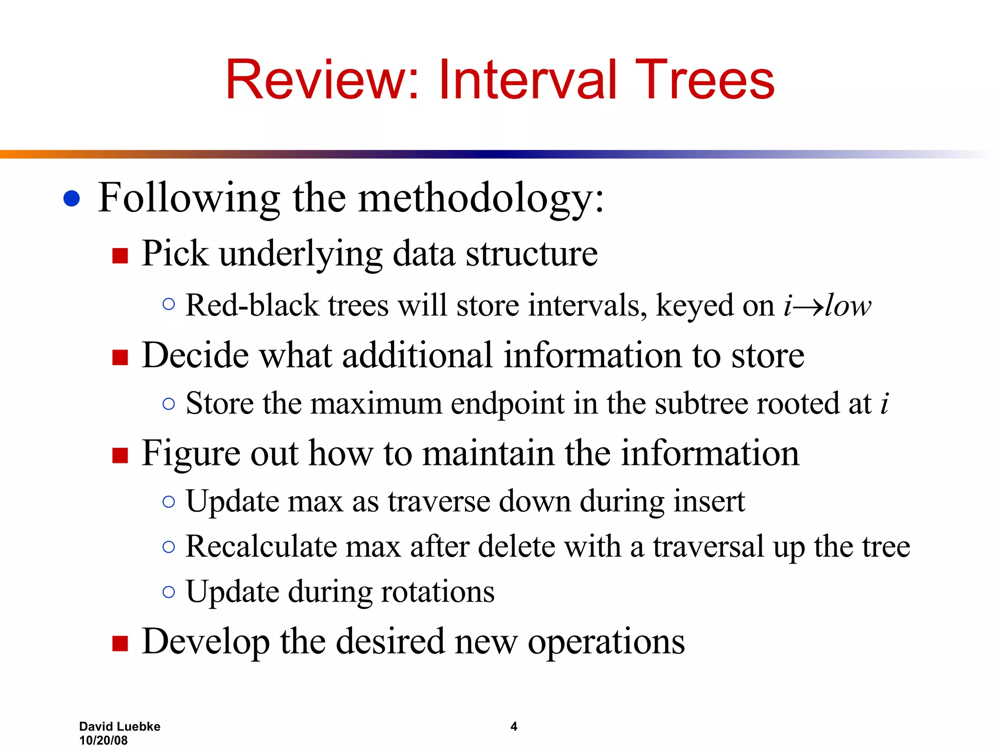
Review: Interval Trees Following the methodology: Pick underlying data structure Red-black trees will store intervals, keyed on i  low Decide what additional information to store Store the maximum endpoint in the subtree rooted at i Figure out how to maintain the information Update max as traverse down during insert Recalculate max after delete with a traversal up the tree Update during rotations Develop the desired new operations

Review: Interval Trees [17,19] 23 [5,11] 18 [21,23] 23 [4,8] 8 [15,18] 18 [7,10] 10 int max Note that:

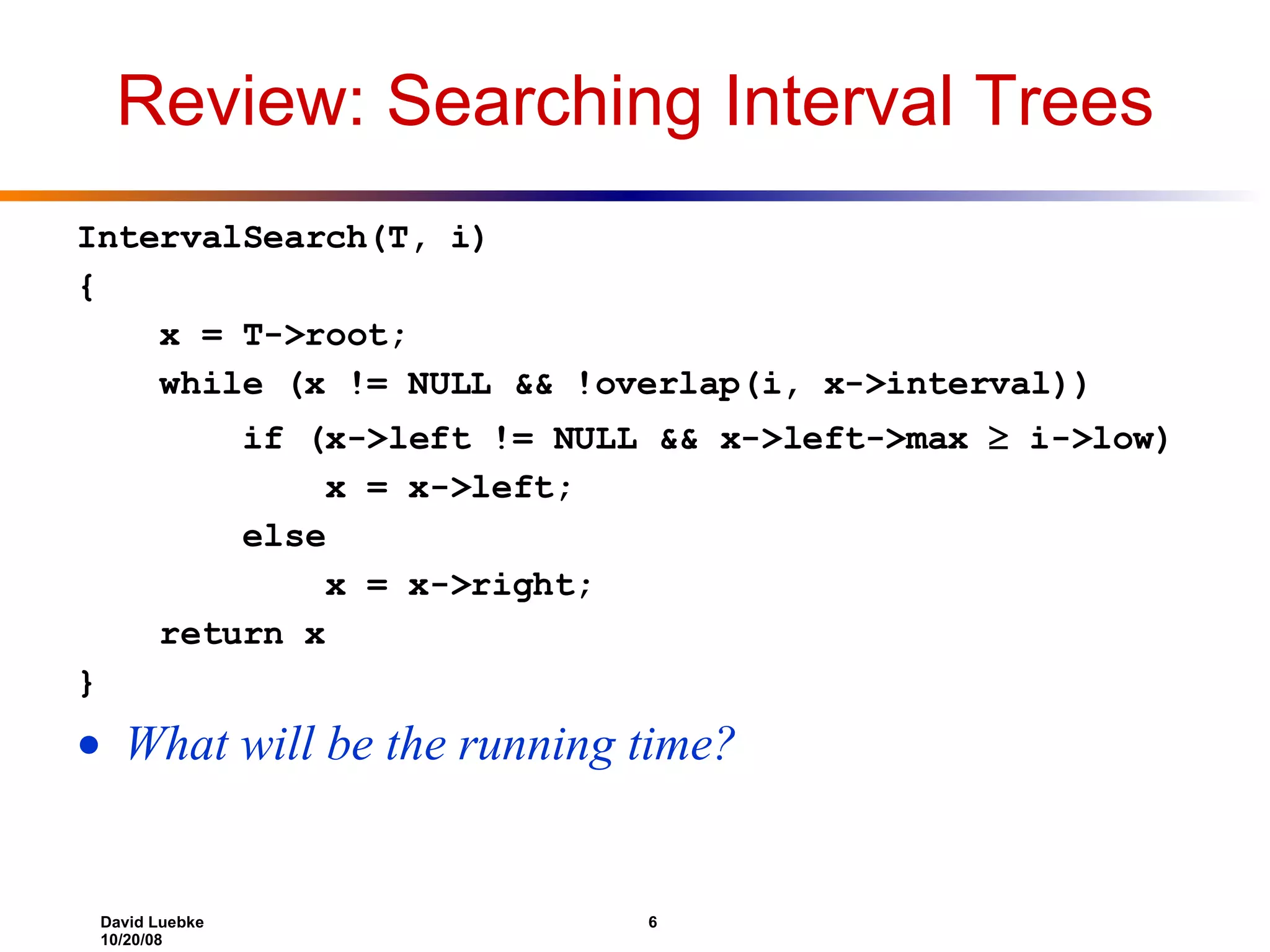
Review: Searching Interval Trees IntervalSearch(T, i) { x = T->root; while (x != NULL && !overlap(i, x->interval)) if (x->left != NULL && x->left->max  i->low) x = x->left; else x = x->right; return x } What will be the running time?

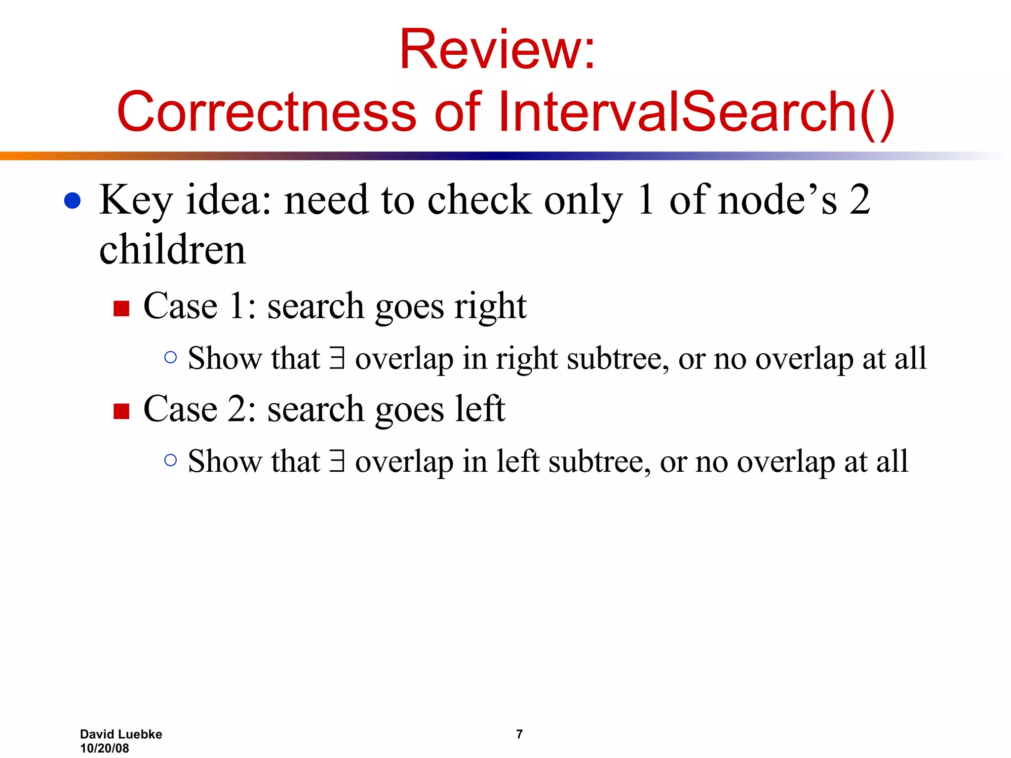
Review: Correctness of IntervalSearch() Key idea: need to check only 1 of node’s 2 children Case 1: search goes right Show that  overlap in right subtree, or no overlap at all Case 2: search goes left Show that  overlap in left subtree, or no overlap at all

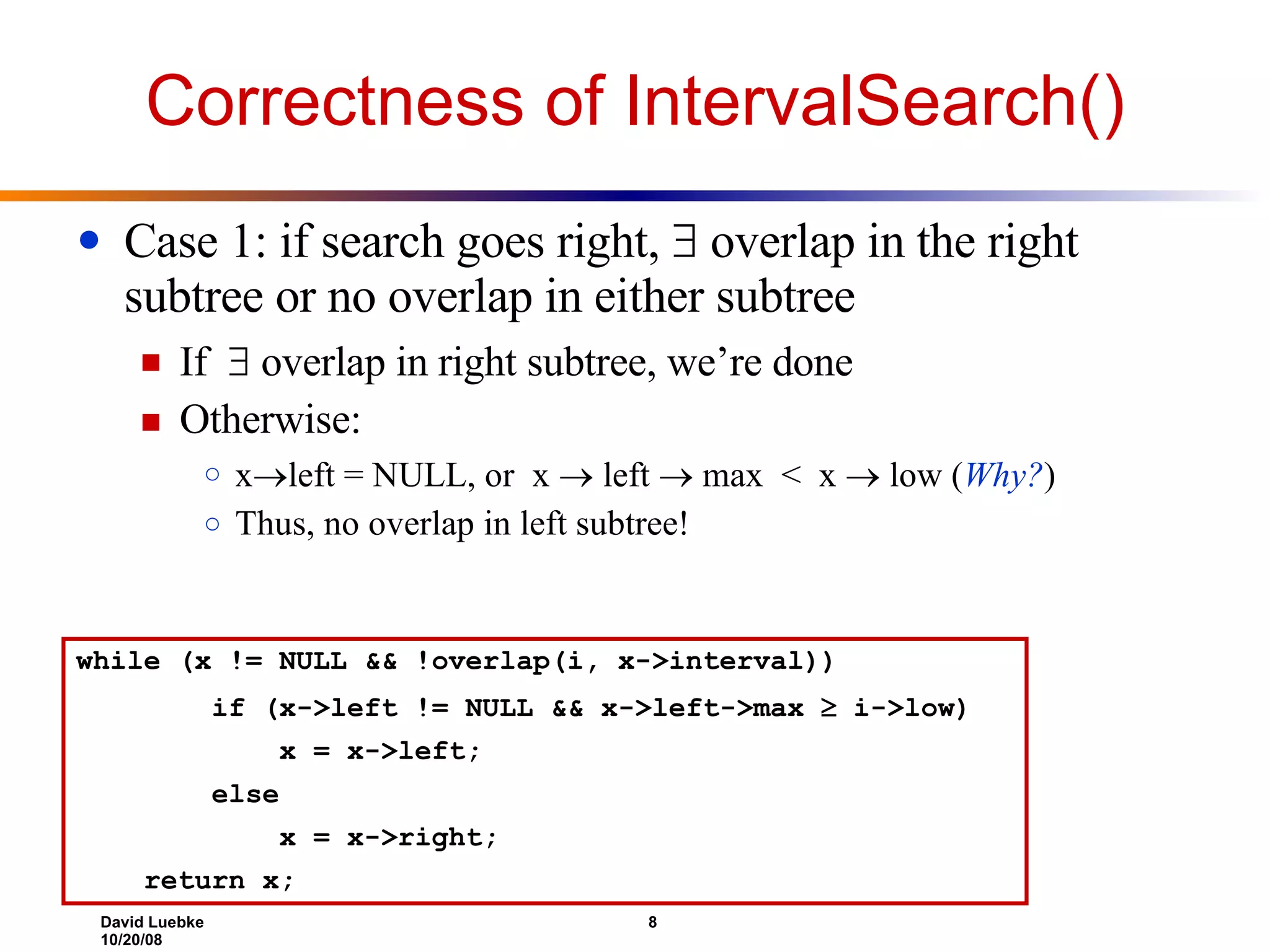
Correctness of IntervalSearch() Case 1: if search goes right,  overlap in the right subtree or no overlap in either subtree If  overlap in right subtree, we’re done Otherwise: x  left = NULL, or x  left  max < x  low ( Why? ) Thus, no overlap in left subtree! while (x != NULL && !overlap(i, x->interval)) if (x->left != NULL && x->left->max  i->low) x = x->left; else x = x->right; return x;

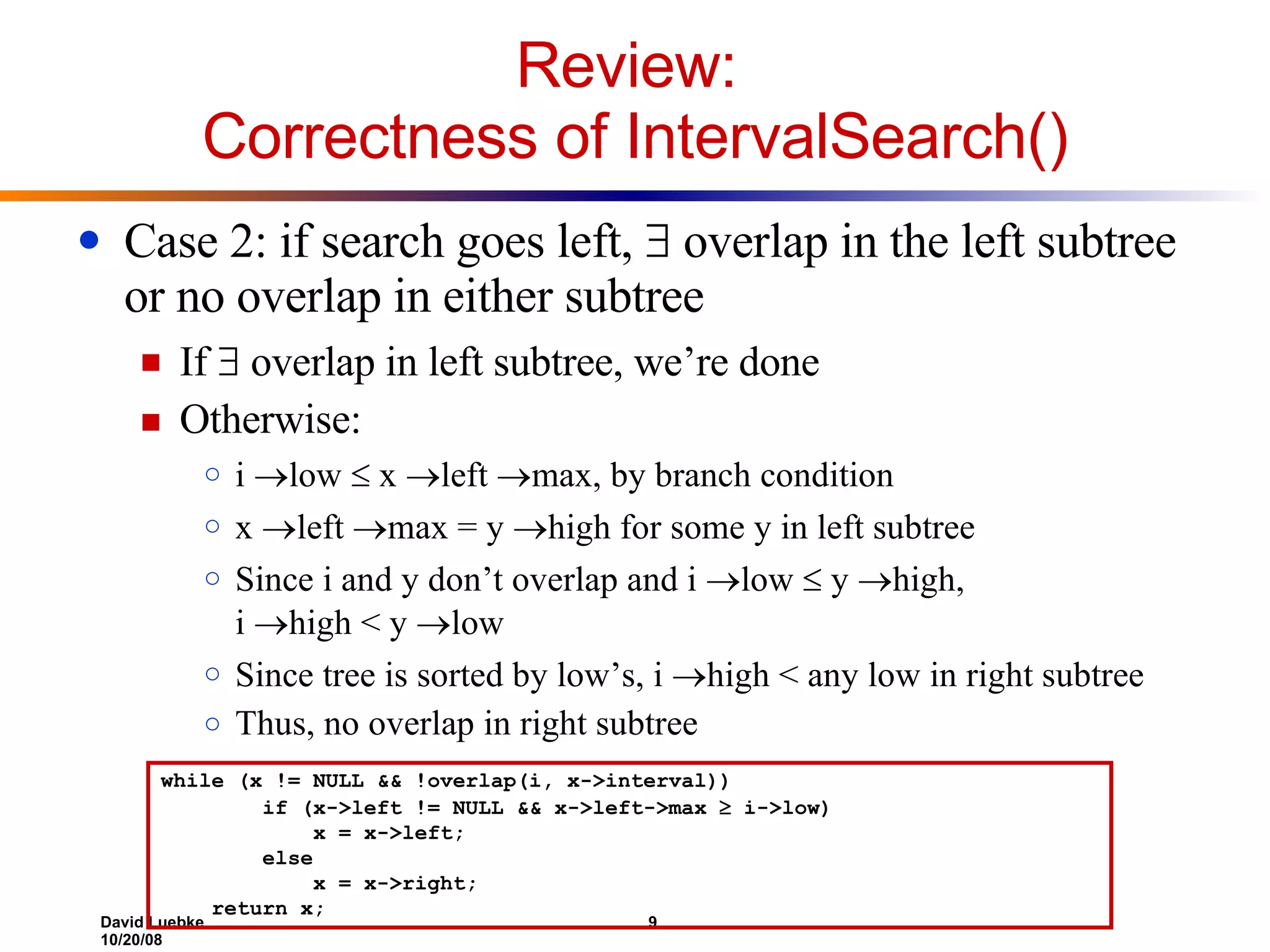
Review: Correctness of IntervalSearch() Case 2: if search goes left,  overlap in the left subtree or no overlap in either subtree If  overlap in left subtree, we’re done Otherwise: i  low  x  left  max, by branch condition x  left  max = y  high for some y in left subtree Since i and y don’t overlap and i  low  y  high, i  high < y  low Since tree is sorted by low’s, i  high < any low in right subtree Thus, no overlap in right subtree while (x != NULL && !overlap(i, x->interval)) if (x->left != NULL && x->left->max  i->low) x = x->left; else x = x->right; return x;

Next Up: Graph Algorithms Going to skip some advanced data structures B-Trees Balanced search tree designed to minimize disk I/O Fibonacci heaps Heap structure that supports efficient “merge heap” op Requires amortized analysis techniques Will hopefully return to these Meantime: graph algorithms Should be largely review, easier for exam

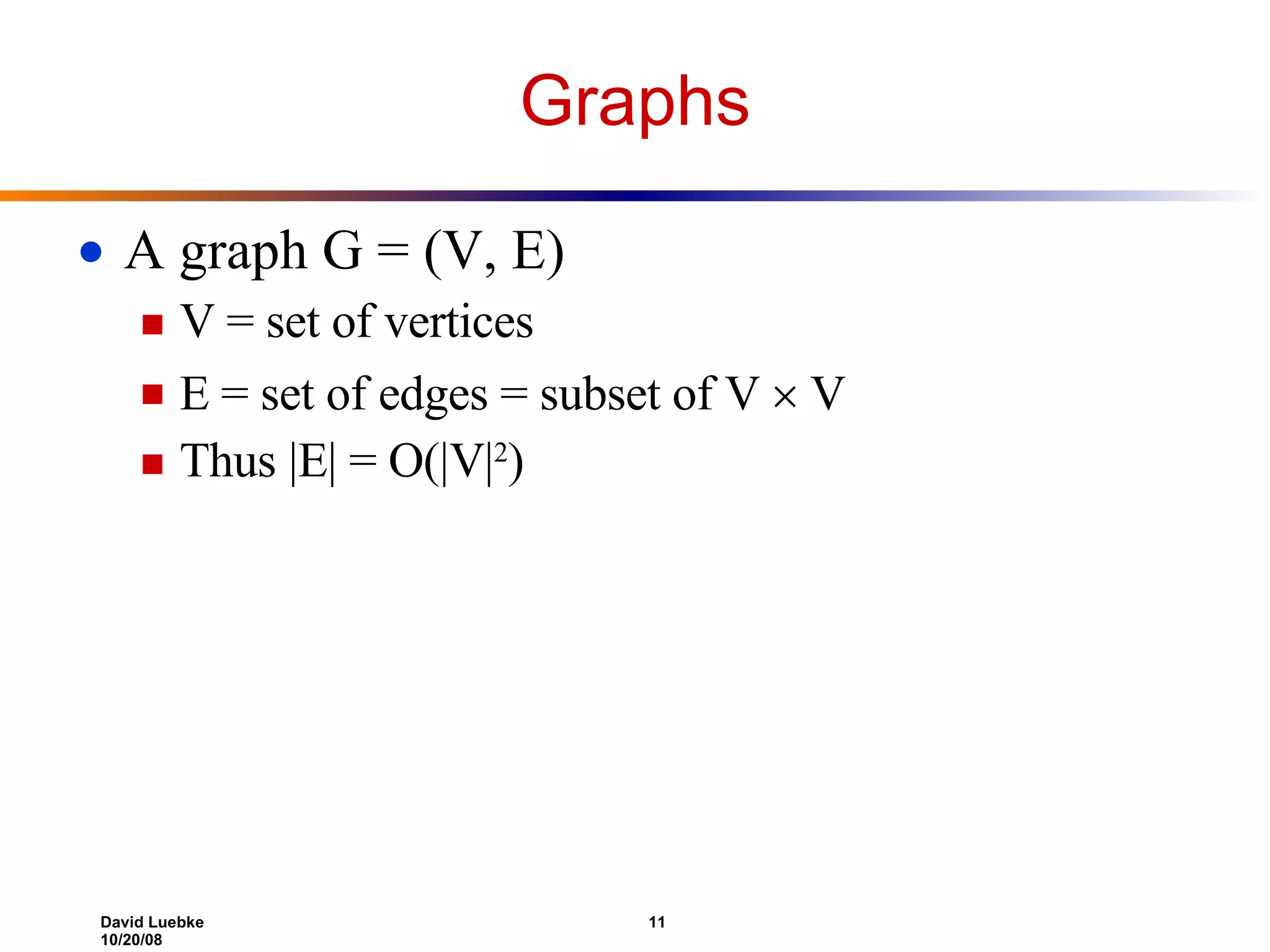
Graphs A graph G = (V, E) V = set of vertices E = set of edges = subset of V  V Thus |E| = O(|V| 2 )

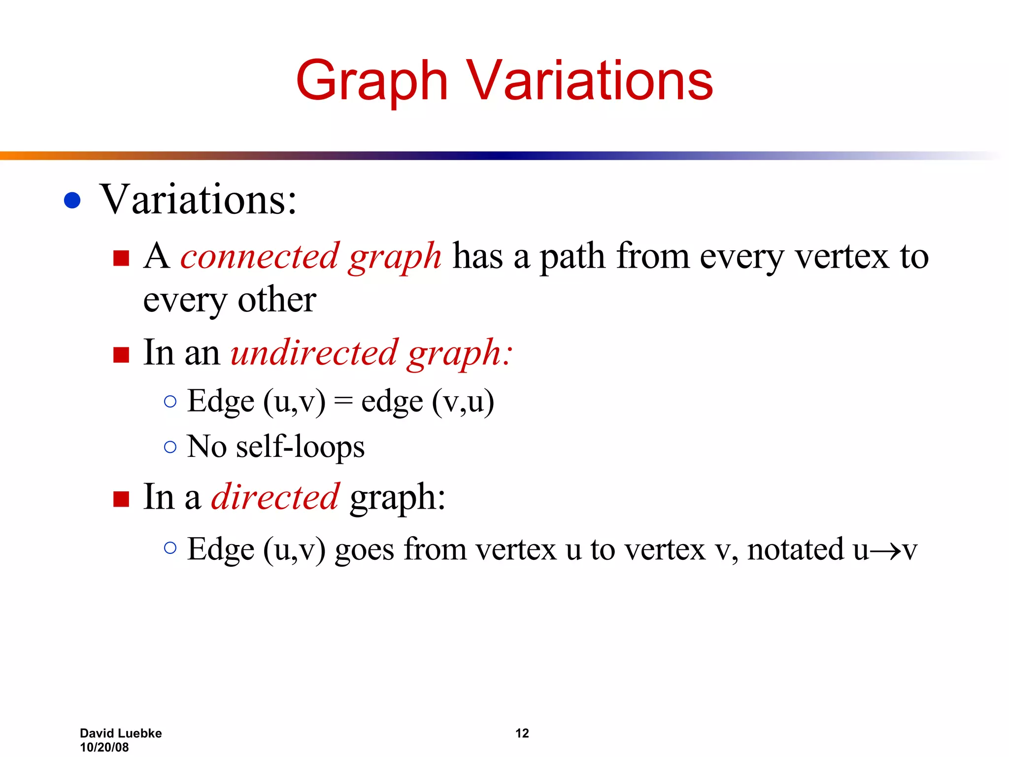
Graph Variations Variations: A connected graph has a path from every vertex to every other In an undirected graph: Edge (u,v) = edge (v,u) No self-loops In a directed graph: Edge (u,v) goes from vertex u to vertex v, notated u  v

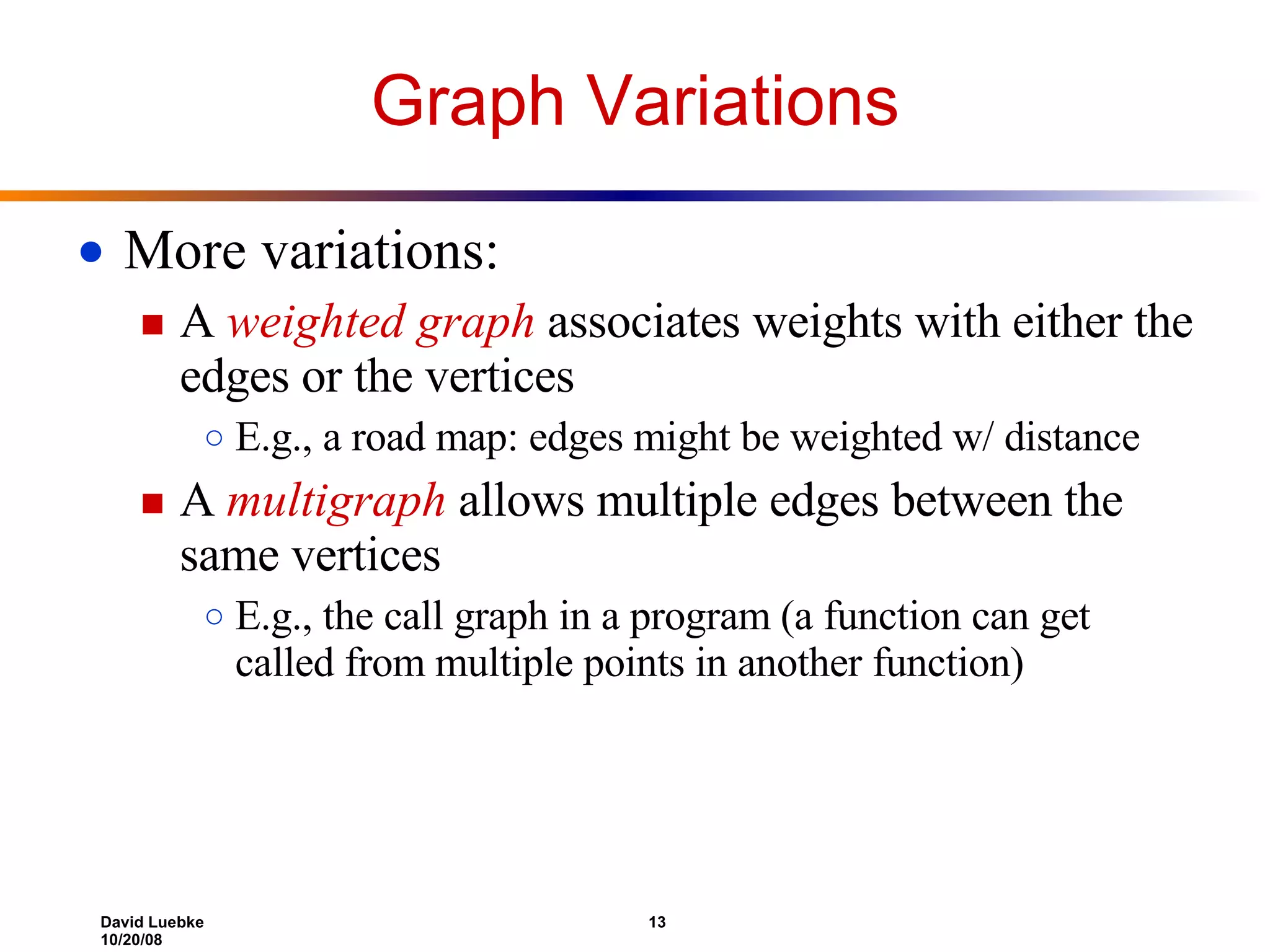
Graph Variations More variations: A weighted graph associates weights with either the edges or the vertices E.g., a road map: edges might be weighted w/ distance A multigraph allows multiple edges between the same vertices E.g., the call graph in a program (a function can get called from multiple points in another function)

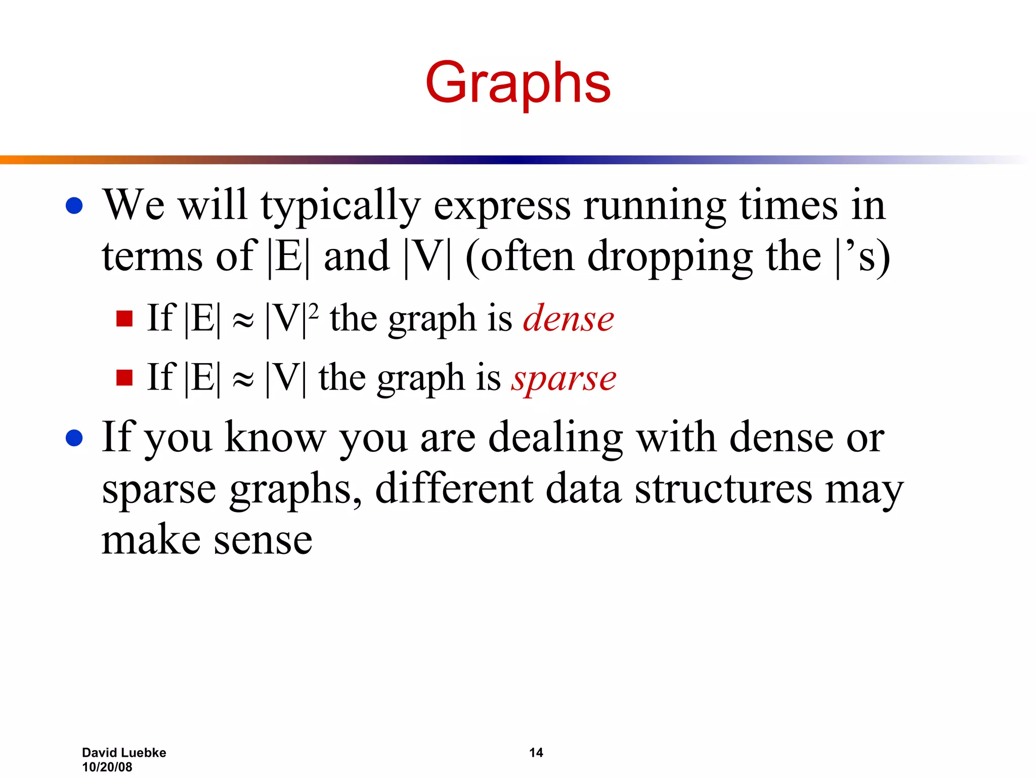
Graphs We will typically express running times in terms of |E| and |V| (often dropping the |’s) If |E|  |V| 2 the graph is dense If |E|  |V| the graph is sparse If you know you are dealing with dense or sparse graphs, different data structures may make sense

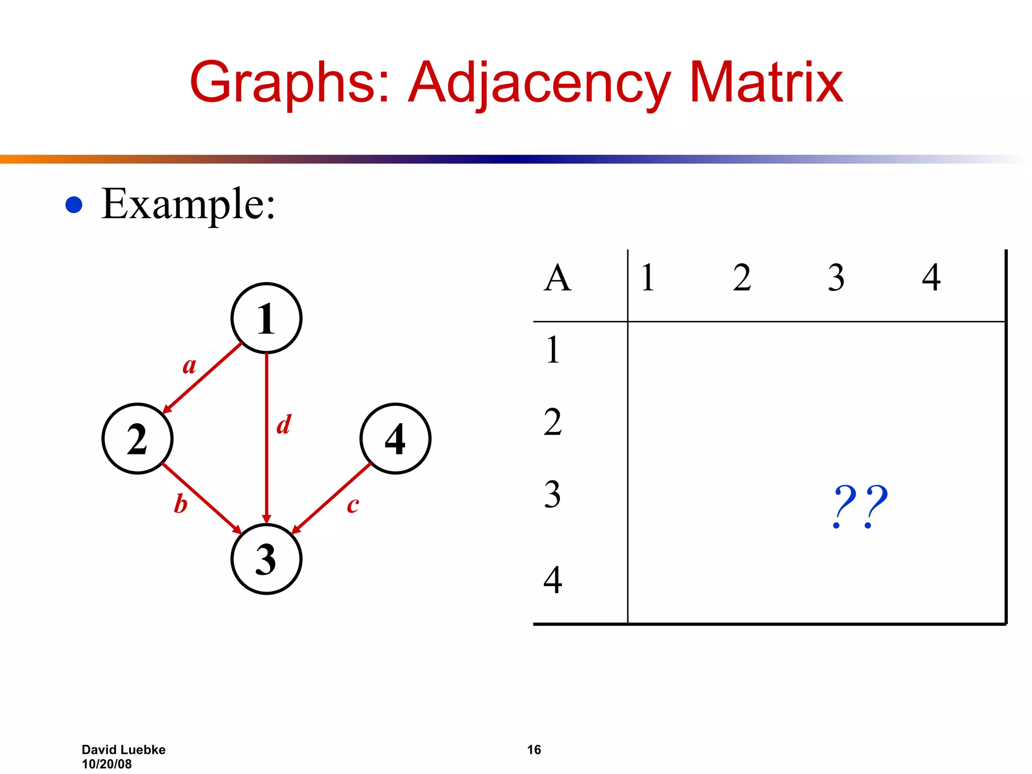
Representing Graphs Assume V = {1, 2, …, n } An adjacency matrix represents the graph as a n x n matrix A: A[ i , j ] = 1 if edge ( i , j )  E (or weight of edge) = 0 if edge ( i , j )  E

Graphs: Adjacency Matrix Example: 1 2 4 3 a d b c 4 ?? 3 2 1 4 3 2 1 A

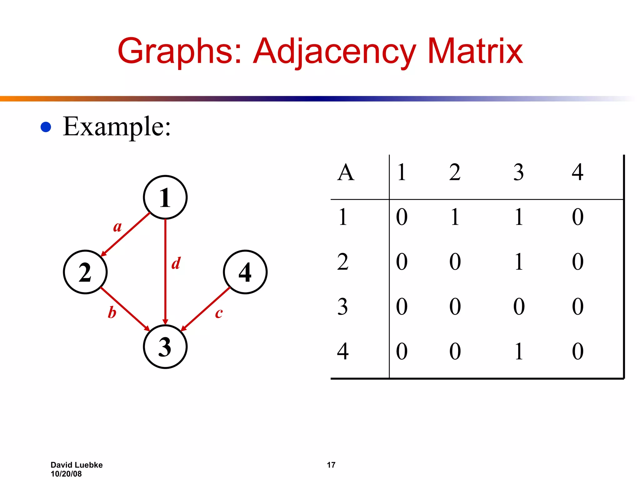
Graphs: Adjacency Matrix Example: 1 2 4 3 a d b c 0 1 0 0 4 0 0 0 0 3 0 1 0 0 2 0 1 1 0 1 4 3 2 1 A

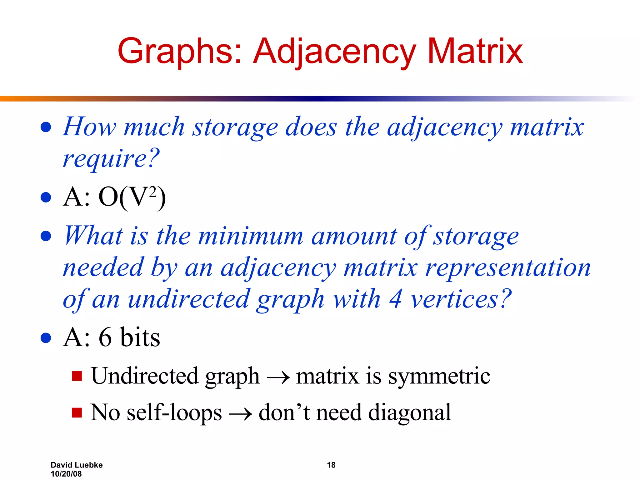
Graphs: Adjacency Matrix How much storage does the adjacency matrix require? A: O(V 2 ) What is the minimum amount of storage needed by an adjacency matrix representation of an undirected graph with 4 vertices? A: 6 bits Undirected graph  matrix is symmetric No self-loops  don’t need diagonal

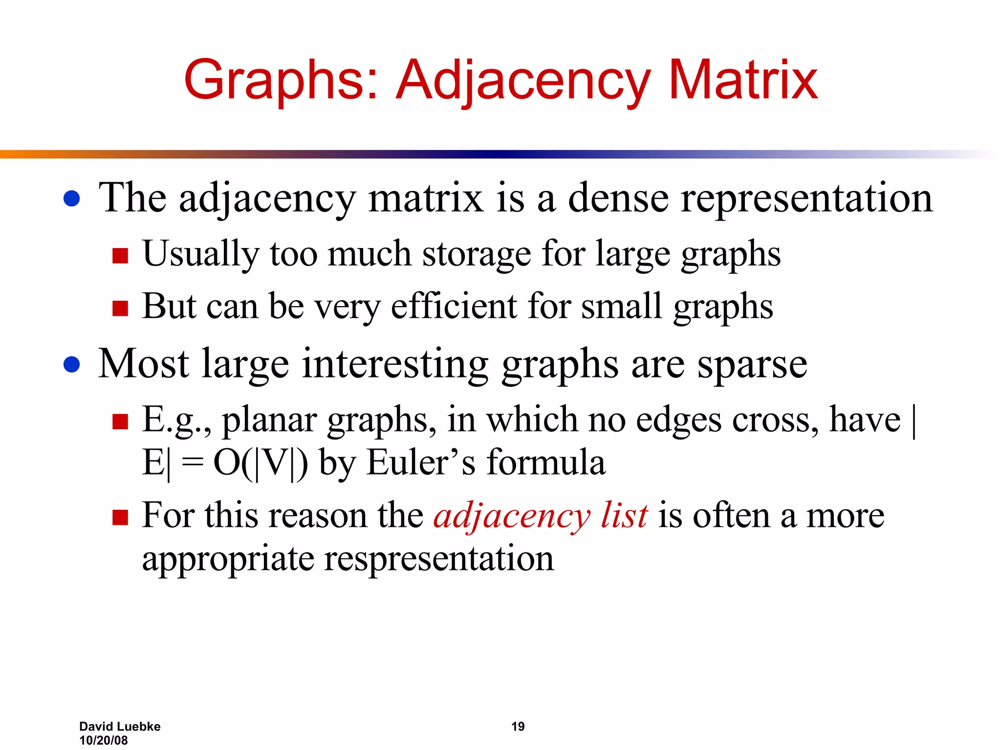
Graphs: Adjacency Matrix The adjacency matrix is a dense representation Usually too much storage for large graphs But can be very efficient for small graphs Most large interesting graphs are sparse E.g., planar graphs, in which no edges cross, have |E| = O(|V|) by Euler’s formula For this reason the adjacency list is often a more appropriate respresentation

Graphs: Adjacency List Adjacency list: for each vertex v  V, store a list of vertices adjacent to v Example: Adj[1] = {2,3} Adj[2] = {3} Adj[3] = {} Adj[4] = {3} Variation: can also keep a list of edges coming into vertex 1 2 4 3

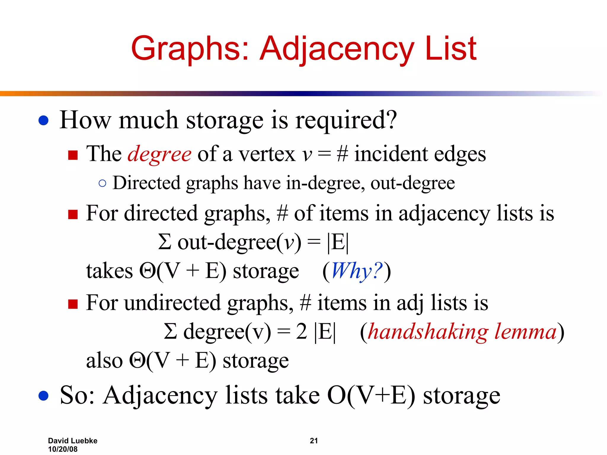
Graphs: Adjacency List How much storage is required? The degree of a vertex v = # incident edges Directed graphs have in-degree, out-degree For directed graphs, # of items in adjacency lists is  out-degree( v ) = |E| takes  (V + E) storage ( Why? ) For undirected graphs, # items in adj lists is  degree(v) = 2 |E| ( handshaking lemma ) also  (V + E) storage So: Adjacency lists take O(V+E) storage

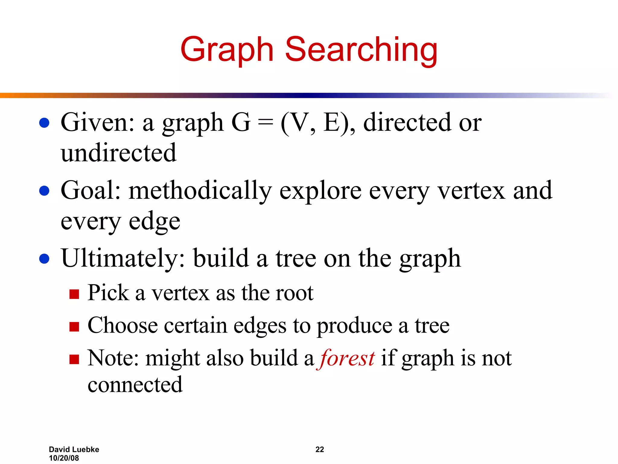
Graph Searching Given: a graph G = (V, E), directed or undirected Goal: methodically explore every vertex and every edge Ultimately: build a tree on the graph Pick a vertex as the root Choose certain edges to produce a tree Note: might also build a forest if graph is not connected

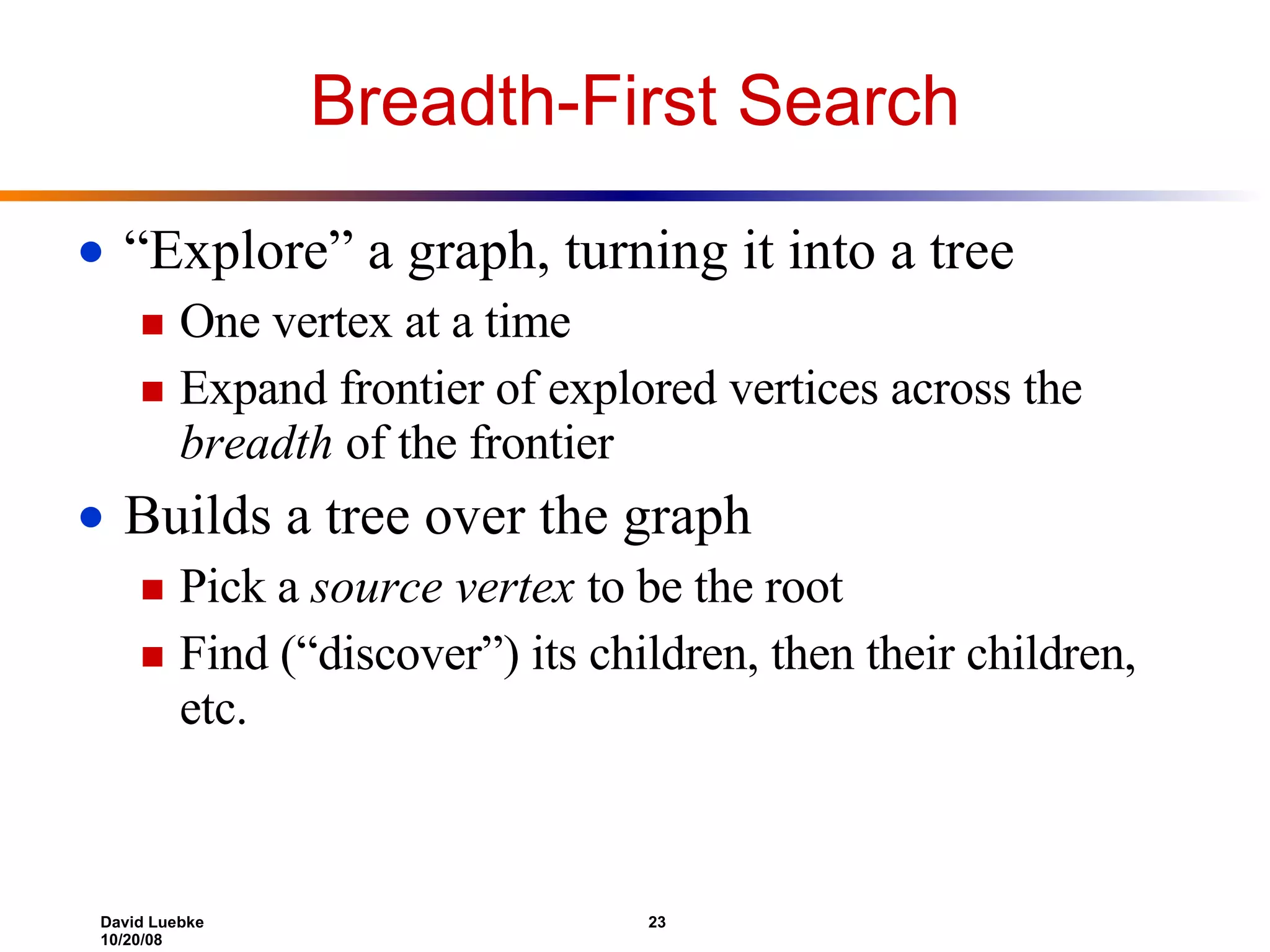
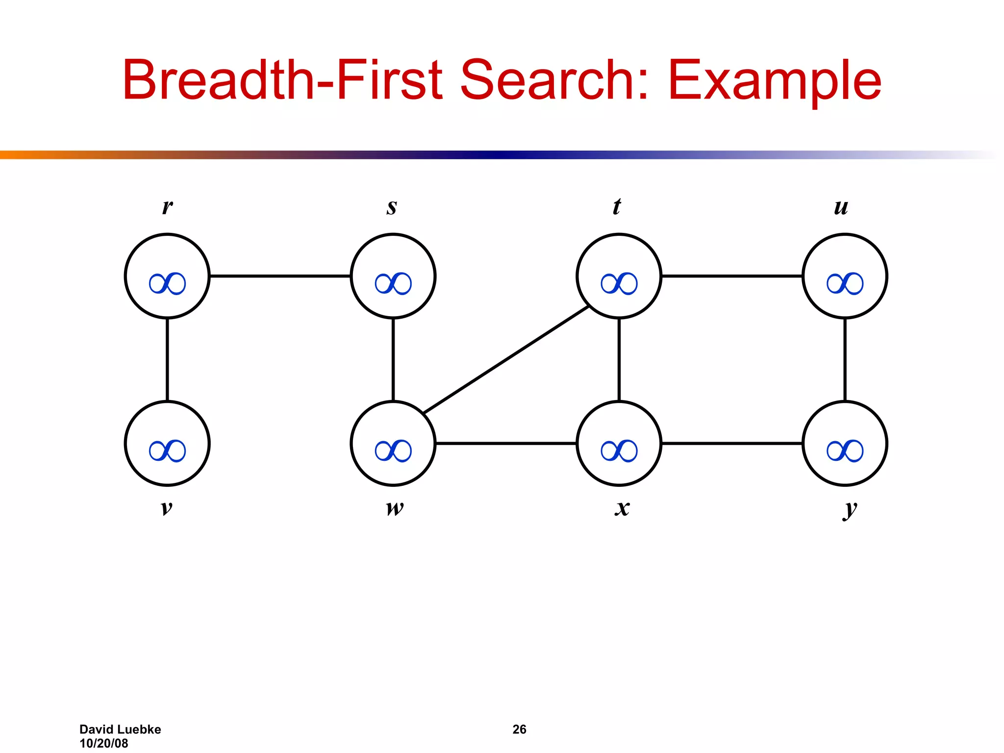
Breadth-First Search “Explore” a graph, turning it into a tree One vertex at a time Expand frontier of explored vertices across the breadth of the frontier Builds a tree over the graph Pick a source vertex to be the root Find (“discover”) its children, then their children, etc.

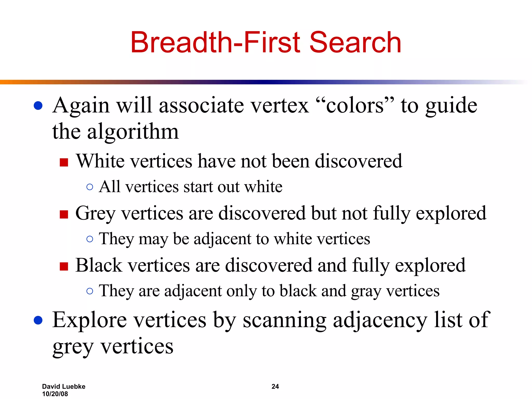
Breadth-First Search Again will associate vertex “colors” to guide the algorithm White vertices have not been discovered All vertices start out white Grey vertices are discovered but not fully explored They may be adjacent to white vertices Black vertices are discovered and fully explored They are adjacent only to black and gray vertices Explore vertices by scanning adjacency list of grey vertices

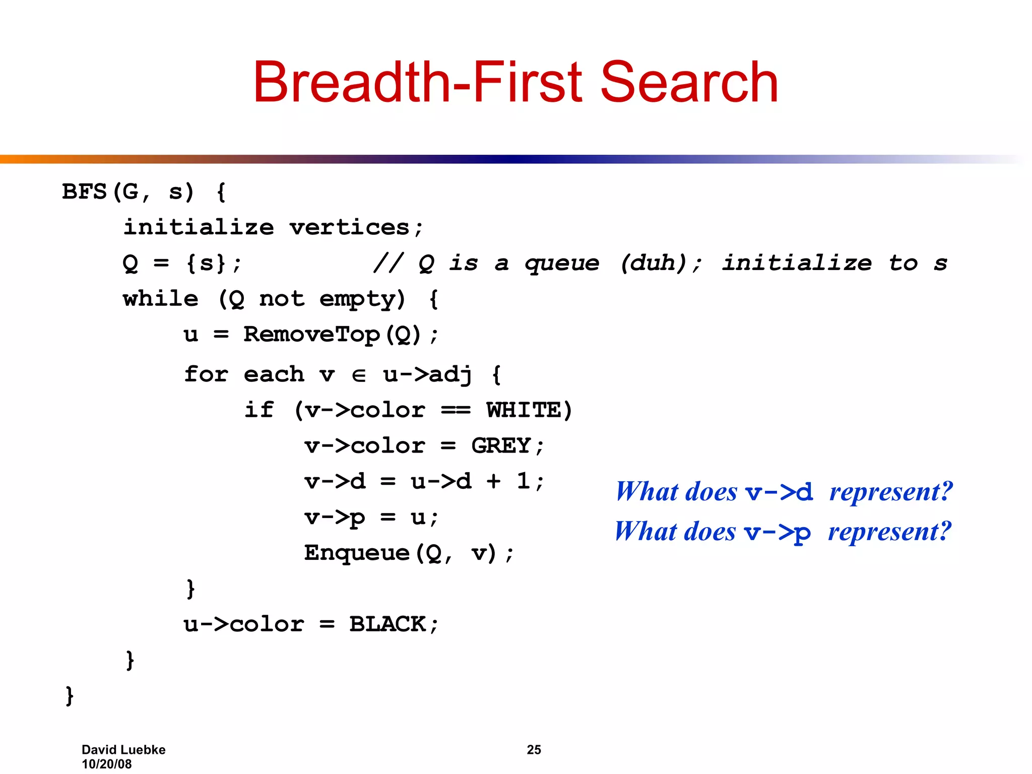
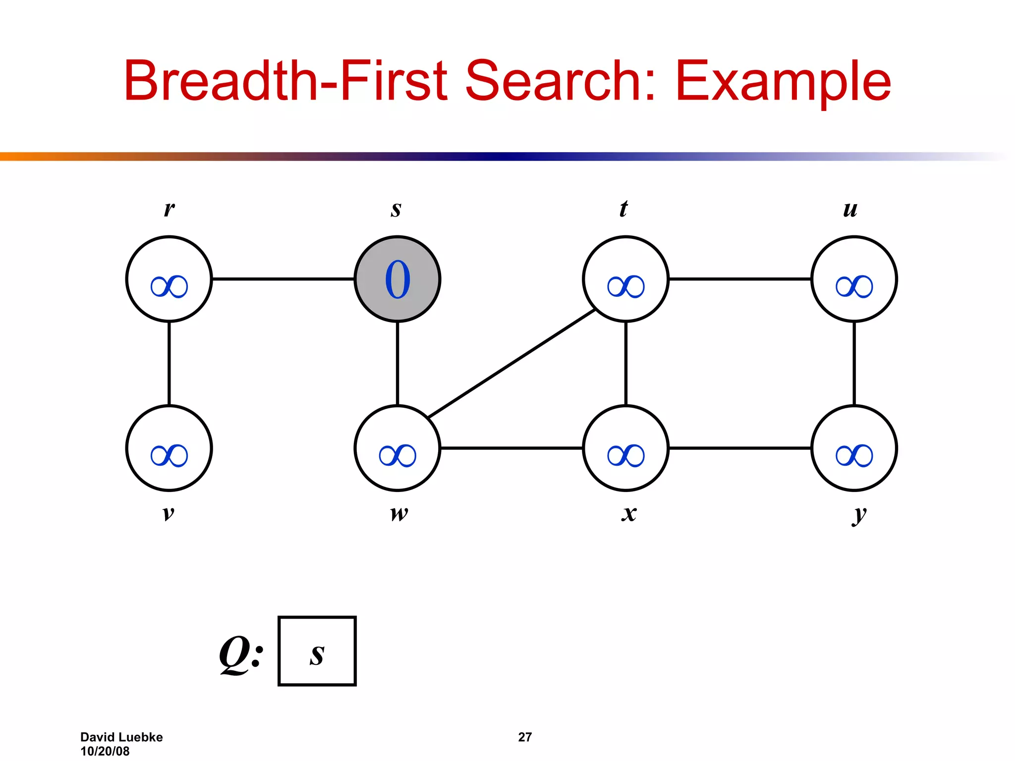
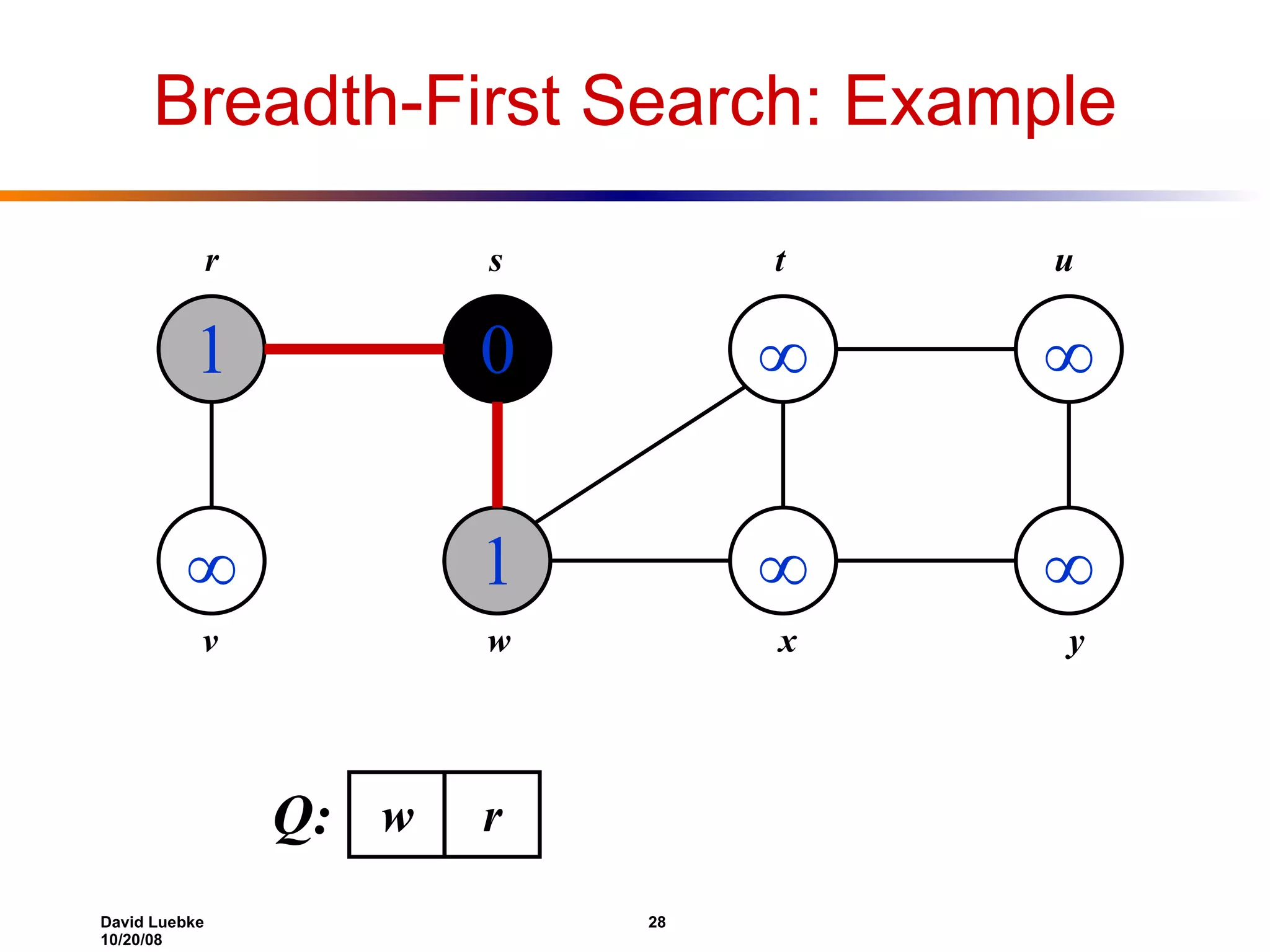
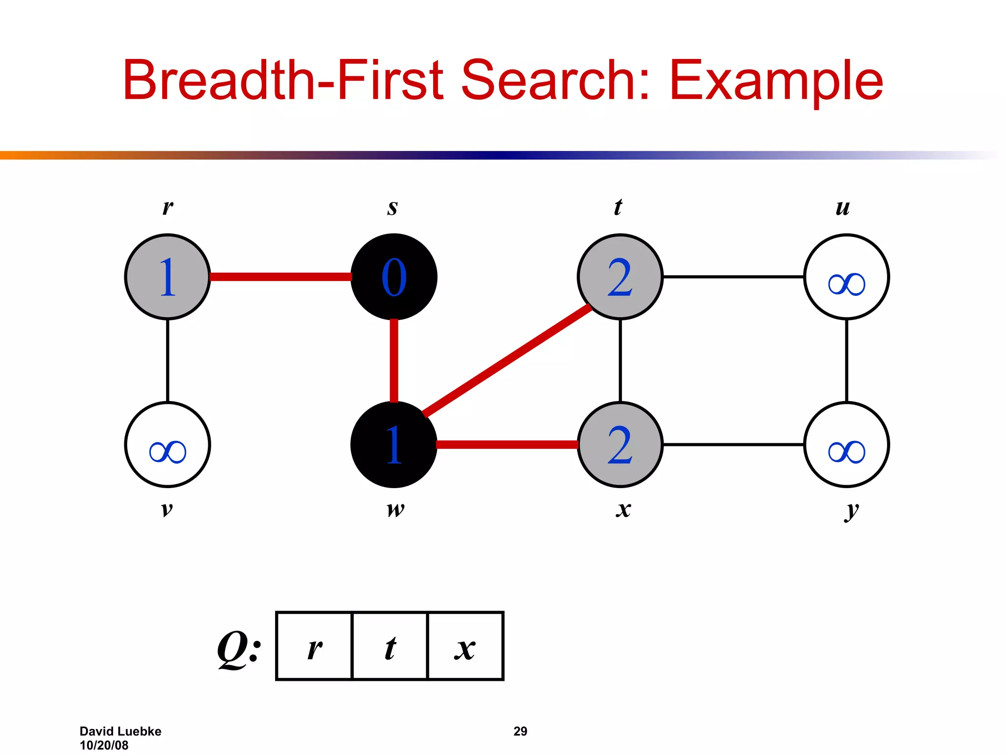
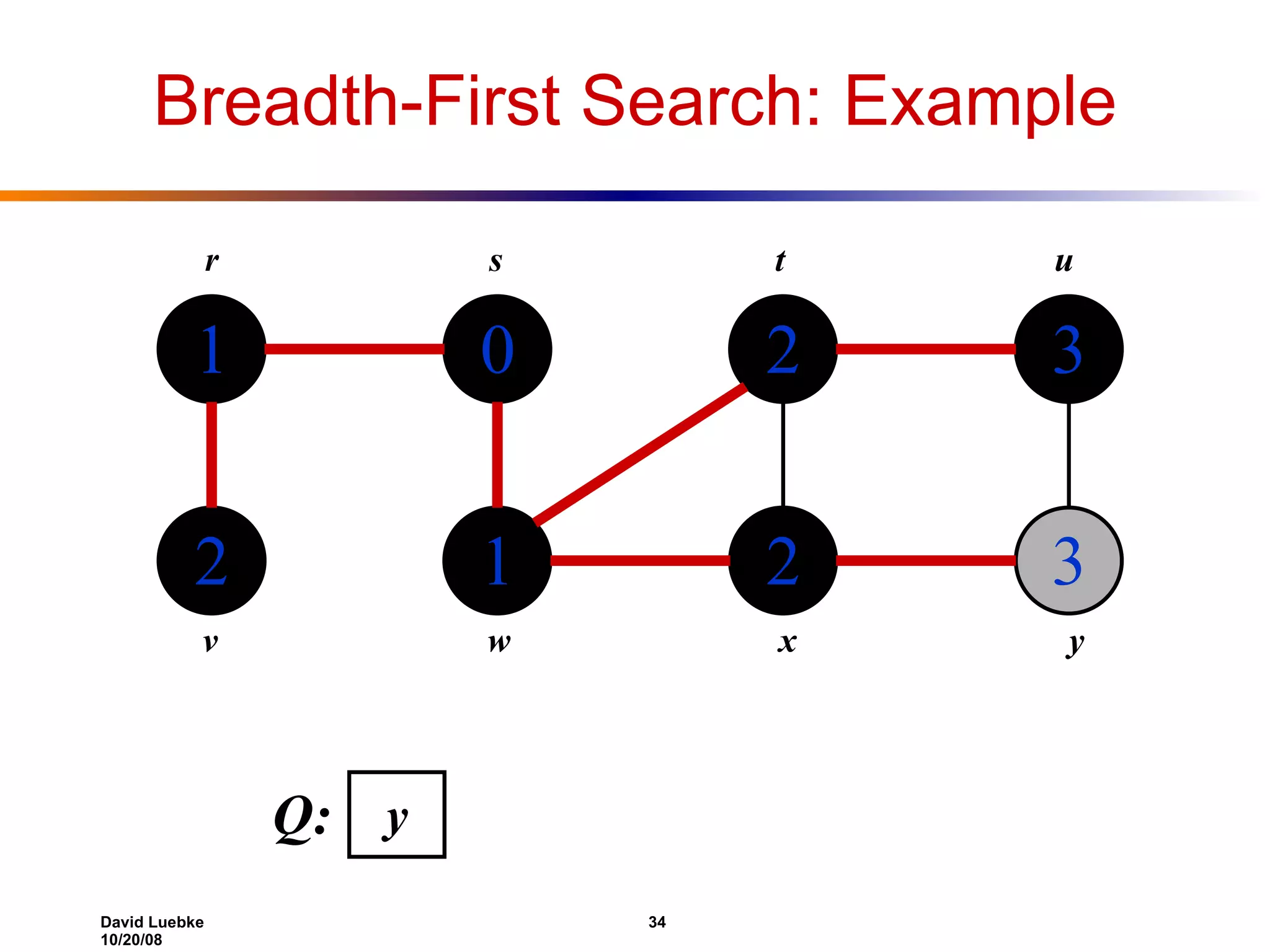
Breadth-First Search BFS(G, s) { initialize vertices; Q = {s}; // Q is a queue (duh); initialize to s while (Q not empty) { u = RemoveTop(Q); for each v  u->adj { if (v->color == WHITE) v->color = GREY; v->d = u->d + 1; v->p = u; Enqueue(Q, v); } u->color = BLACK; } } What does v->p represent? What does v->d represent?

Breadth-First Search: Example         r s t u v w x y

Breadth-First Search: Example   0      r s t u v w x y s Q:

Breadth-First Search: Example 1  0 1     r s t u v w x y w Q: r

Breadth-First Search: Example 1  0 1 2 2   r s t u v w x y r Q: t x

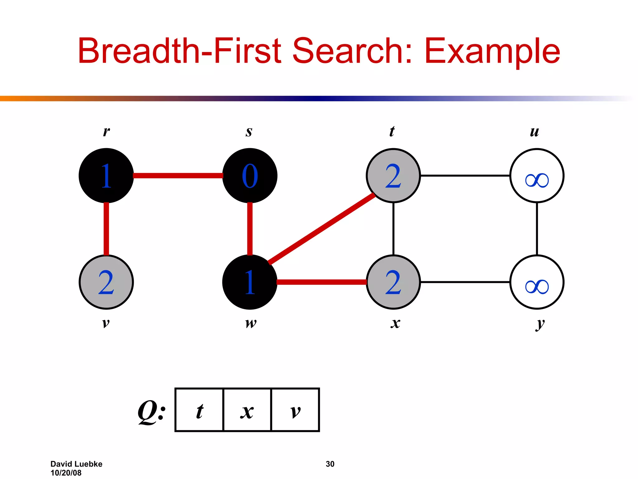
Breadth-First Search: Example 1 2 0 1 2 2   r s t u v w x y Q: t x v

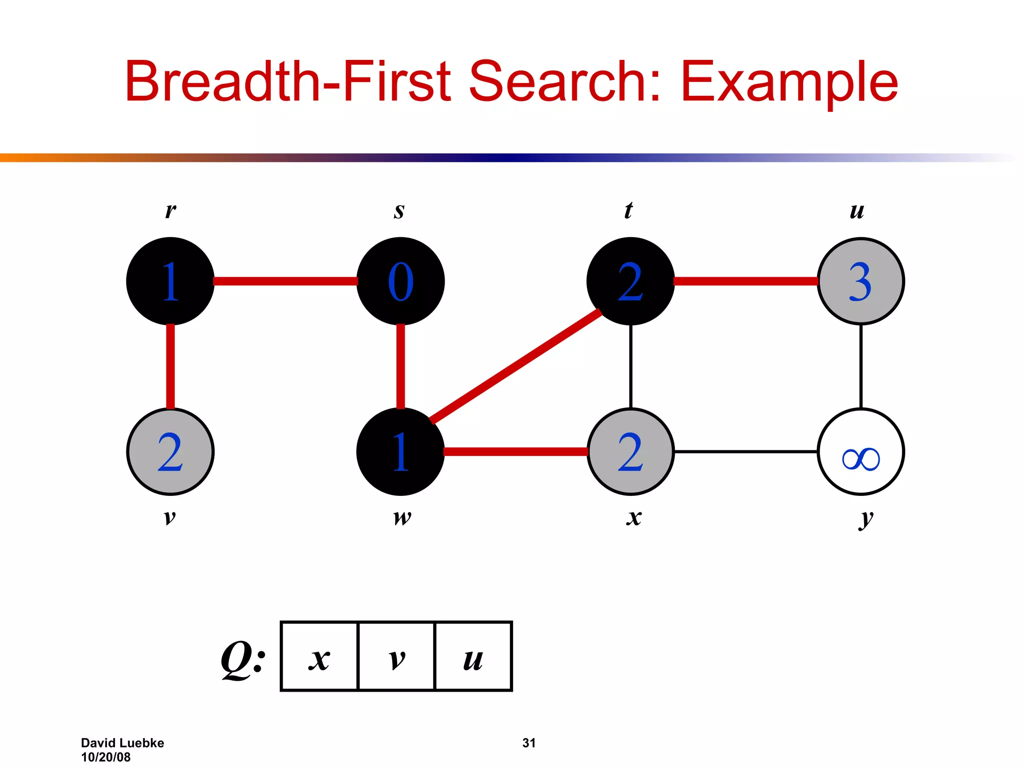
Breadth-First Search: Example 1 2 0 1 2 2 3  r s t u v w x y Q: x v u

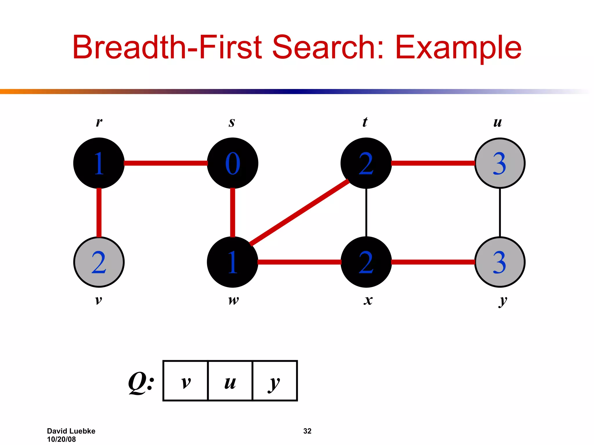
Breadth-First Search: Example 1 2 0 1 2 2 3 3 r s t u v w x y Q: v u y

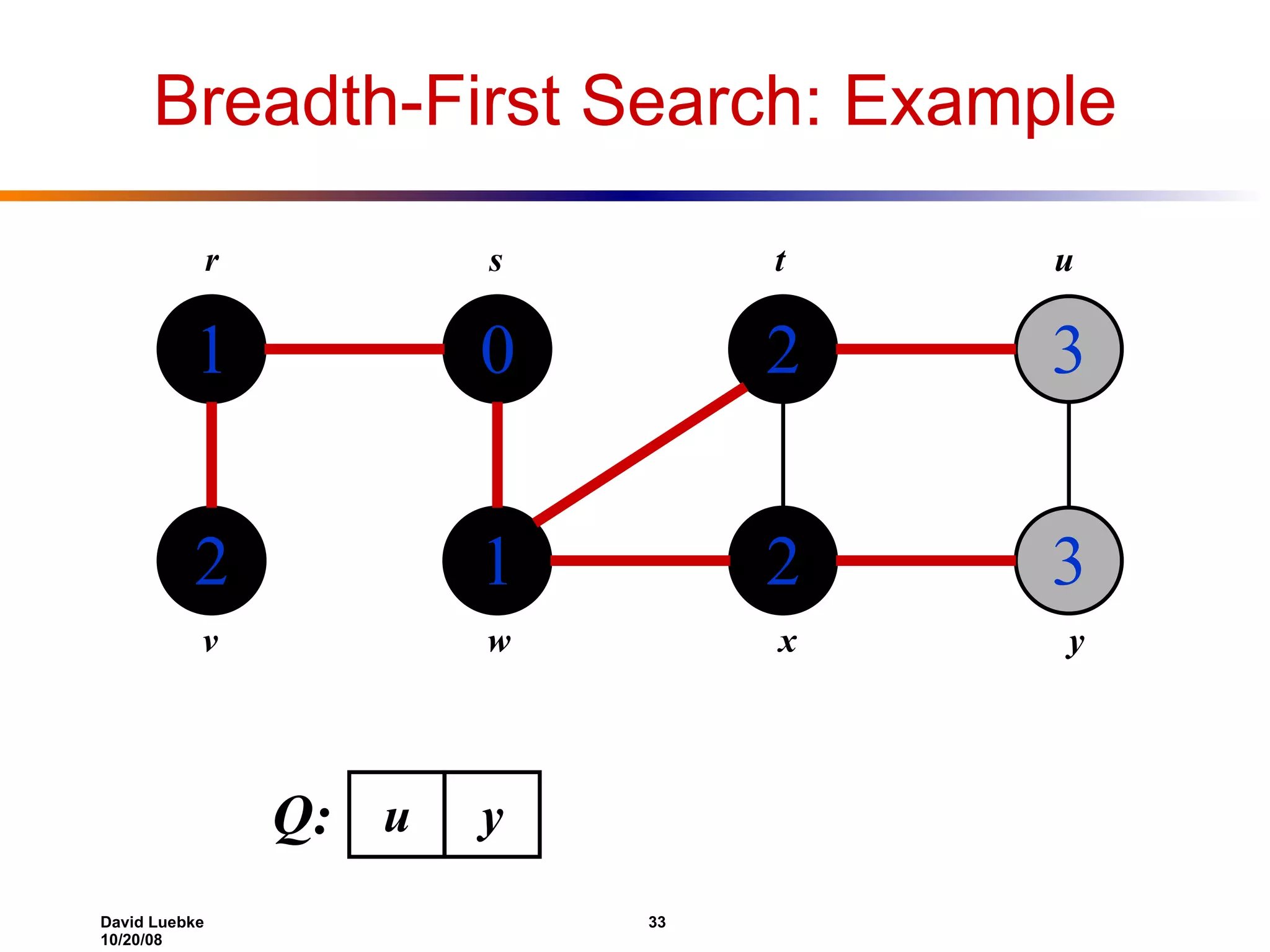
Breadth-First Search: Example 1 2 0 1 2 2 3 3 r s t u v w x y Q: u y

Breadth-First Search: Example 1 2 0 1 2 2 3 3 r s t u v w x y Q: y

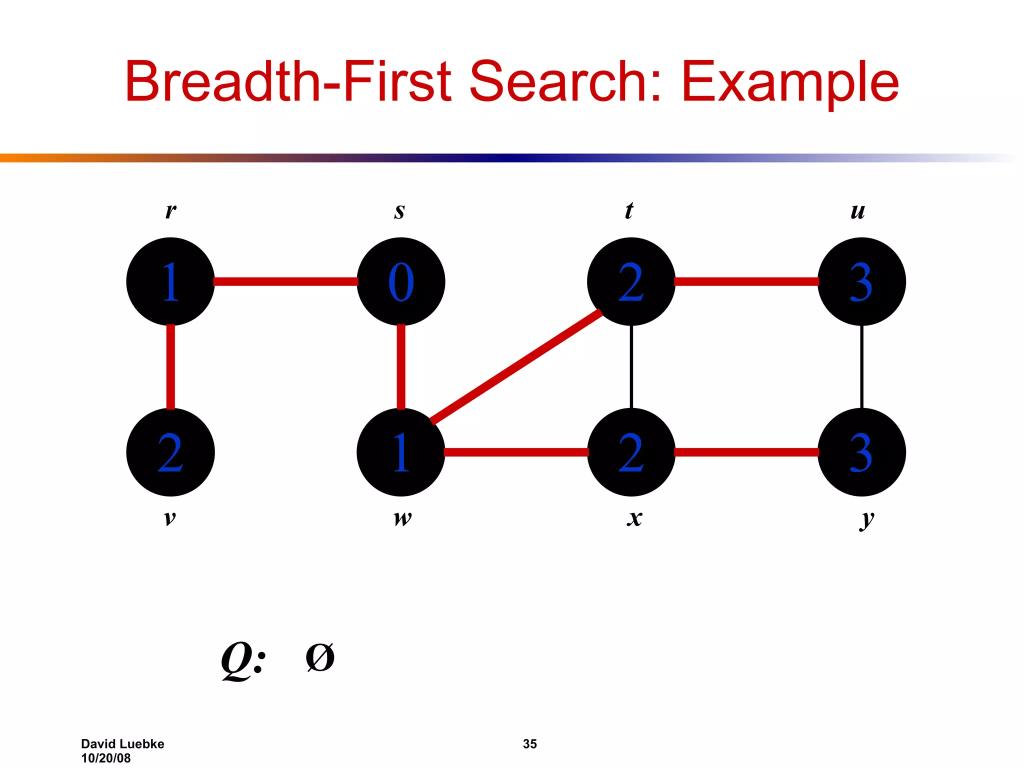
Breadth-First Search: Example 1 2 0 1 2 2 3 3 r s t u v w x y Q: Ø

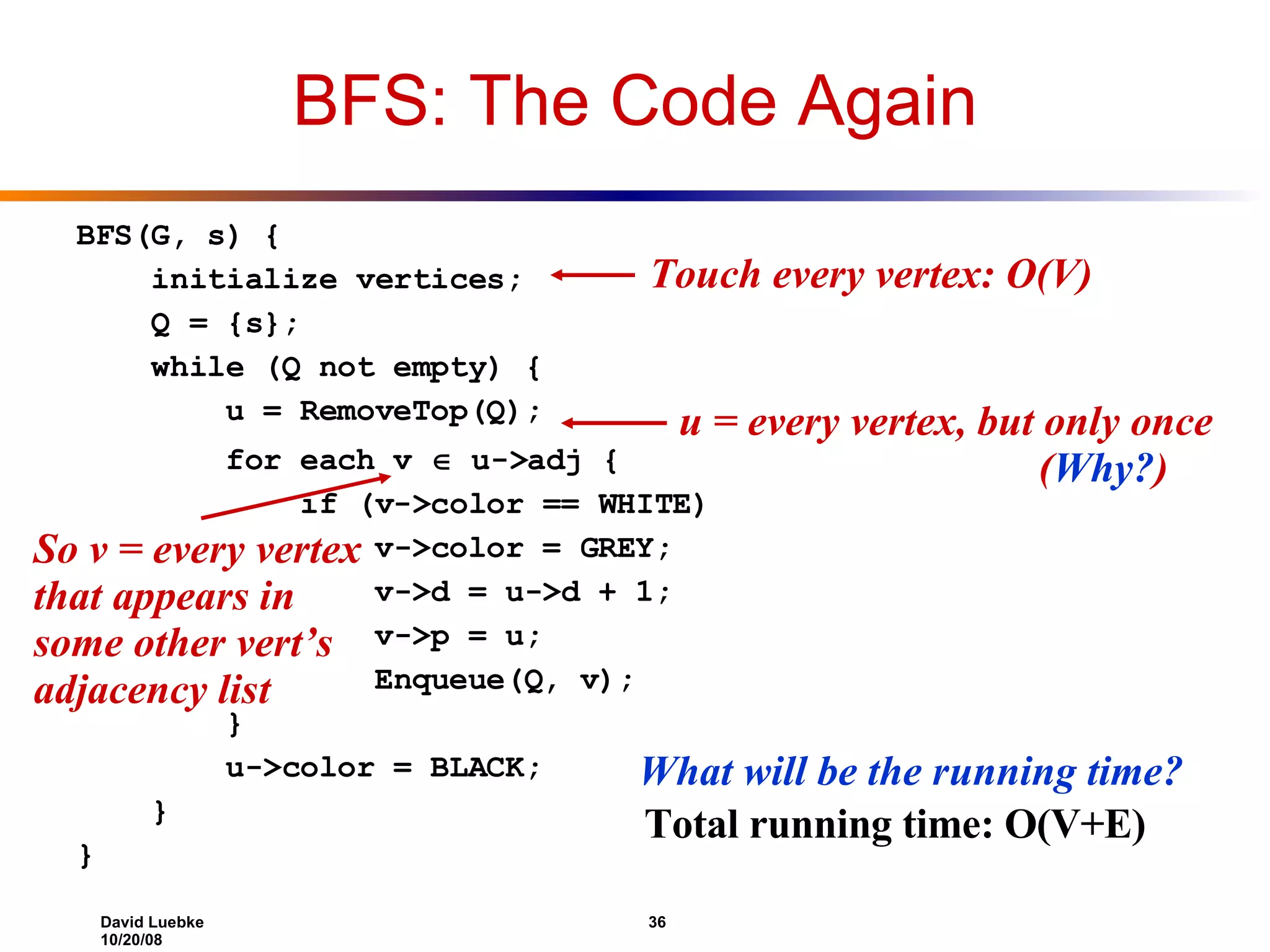
BFS: The Code Again BFS(G, s) { initialize vertices; Q = {s}; while (Q not empty) { u = RemoveTop(Q); for each v  u->adj { if (v->color == WHITE) v->color = GREY; v->d = u->d + 1; v->p = u; Enqueue(Q, v); } u->color = BLACK; } } What will be the running time? Total running time: O(V+E) Touch every vertex: O(V) u = every vertex, but only once ( Why? ) So v = every vertex that appears in some other vert’s adjacency list

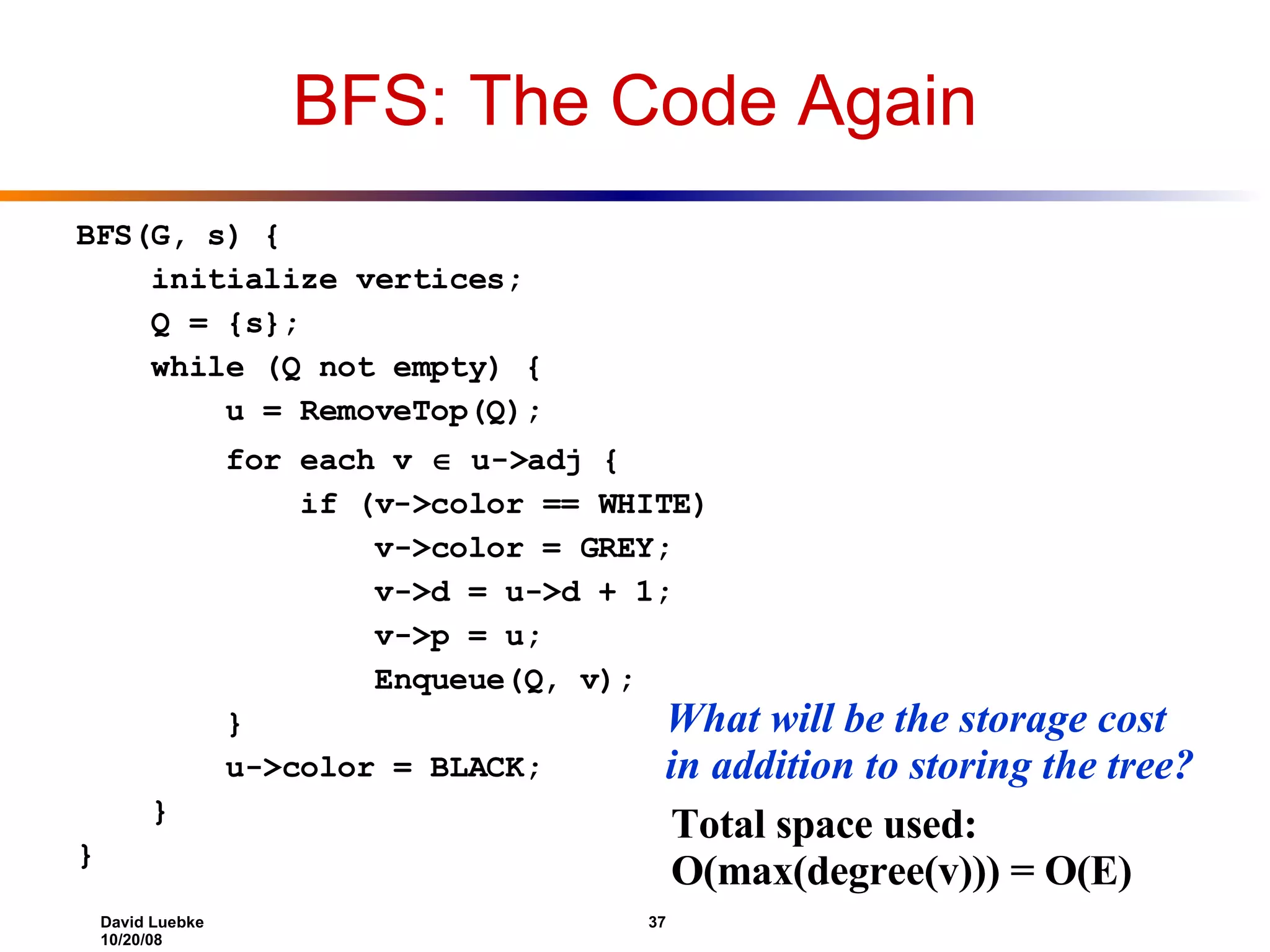
BFS: The Code Again BFS(G, s) { initialize vertices; Q = {s}; while (Q not empty) { u = RemoveTop(Q); for each v  u->adj { if (v->color == WHITE) v->color = GREY; v->d = u->d + 1; v->p = u; Enqueue(Q, v); } u->color = BLACK; } } What will be the storage cost in addition to storing the tree? Total space used: O(max(degree(v))) = O(E)

Breadth-First Search: Properties BFS calculates the shortest-path distance to the source node Shortest-path distance  (s,v) = minimum number of edges from s to v, or  if v not reachable from s Proof given in the book (p. 472-5) BFS builds breadth-first tree , in which paths to root represent shortest paths in G Thus can use BFS to calculate shortest path from one vertex to another in O(V+E) time

lecture 17

More Related Content

What's hot

Viewers also liked

Similar to lecture 17

More from sajinsc

Recently uploaded

lecture 17