Lecture 5 - Linear Regression Linear Regression

Lecture V – Linear Regression

Refresher: Data Models • What is a (mathematical) model?

Refresher: Data Models • What is a (mathematical) model? – useful approximate representation of phenomena that generate data and may be used for prediction, classification, compression, or control design. • How do we obtain these models? – mathematical models of biological or chemical processes etc.? • can be obtained from the principles and laws of physics that govern the process behavior. – Data processing (mining) scenarios? • We find a mathematical model by processing existing data • “black-box” models – How to design? è try to fit the data by using well-known mathematical functions, for example, the function defining a line. • Regression analysis è a data analysis and model discovery process of designing a model of data based on a sample from a given population • Model design consists of: – finding a model structure – computing optimal values of model parameters, – and assessing the model quality

Refresher: Data Models • Model design consists of: – finding a model structure – computing optimal values of model parameters, – and assessing the model quality • A model structure relates to the type (and order in some cases) of mathematical formulas that describe the system behavior – e.g. equations of lines and planes, difference equations, differential equations, Boolean functions etc. • Categories of regression models (depending on the model structure) – Simple linear regression – Multiple linear regression – Neural network-based linear regression (RBF-like models) – Polynomial regression – Logistic regression – Log-linear regression – Local piecewise linear regression – Nonlinear regression (with a nonlinear model) – Neural network-based nonlinear regression

Model Data • Models are designed on available data – Accessible data typically only a sample from total population – Frequently, data space is ‘empty’ since sample is small

A (somewhat complete) ML topology CC content

Refresher: Regression analysis • Statistical method used to: – discover the relationship between variables, and – design a data model that can be used to predict variable values based on other variables (new)

Refresher: Regression analysis • Linear regression è statistical method used to determine the linear relationship and linear data model for two or more variables. • A simple linear regression attempts to find the linear relationship between two variables, x and y, and to discover a linear data model: – a line equation y = b + ax (which is the best fit to given data) in order to predict values of data. – Coefficients b and a are model parameters (b =y- intercept and a = slope/gradient) – Modeling line è regression line of y on x – Linear equation of regression line è regression equation (regression model) • Linear regression attempts to discover the best linear model representing the given dataset (line of best fit), based on a defined performance criterion. E.g. mean squared error – The modelling task is finding a line which is the best fit to a given dataset containing a sample population.

Refresher: Regression error • Since a model is an approximation of the reality, computation of a predicted outcome comes with a certain error. • Let us consider the ith data point xi,yi from the data set T – the predicted variable value computed by the model lies on the regression line: – This value is different from the true data value yi from the data set for data point xi,yi. – This difference e = real-value − predicted-value is the regression error (residual or modelling error)

Recap on Linear Regression • It is a form of supervised learning • Goal = learn a function that predicts a continuous value from a set of training examples – Predicts an outcome variable, or dependent variable – Predicts using a set of independent (explanatory) variables • 1 variable (feature) è univariate (simple) linear regression • 2+ variables (features) è multivariate linear regression • Example problems?

Univariate Linear Regression • Focuses on determining relationship between one independent (explanatory variable) variable and one dependent variable – Input? - data – Task? – fit model – Output? – predicted value of the dependent variable e.g. y from previous slide

Training data m training examples of the form x,y x = independent variable (feature) y = dependent variable (output or target variable – label) e.g. price of a bag of potatoes given rainfall in mms So (xi,yi) refers to the ith training example for i = 1, 2,…..,m X (mm) Y (KES) 50 2500 75 2000 150 2300 10 4000 300 4500 … …

Learning Task • Supervised learning problem: given a training set, learn a function h : X → Y so that h(x) is a “good” predictor for the corresponding value of y • Function è hypothesis (h) • h is a function that maps from x's to y’s

Representing hypothesis h hθ(x) = θ0 + θ1x

Cost function • Used to determine how to fit the best possible straight line to the training data. • Used to measure the accuracy of the hypothesis function hθ(x) • θ0 and θ1 are the parameters of the model. • How do we choose values of θ0 and θ1? – Different values yield different hypothesis functions hθ(x) • Learning goal is to come up with the parameter values that yield a straight line that fits the data ‘well’ – Choose values for parameters θ0 and θ1so that hθ(x) i.e. yest is close to the y values in the training set è minimization problem • Minimize J(θ0,θ1) in hθ(x) = θ0 + θ1x

Cost function: Mean Squared Error (MSE) • Minimize the average distance for each point on the plot from the regression line – If all data points are on the line, what is J(θ0,θ1)? • Choose values for θ0,θ1 that minimize J(θ0,θ1). Note: MSE is halved for convenience when using gradient descent to estimate parameter values

Estimating parameters • How do we choose the best values for θ0 and θ1? è parameter learning – This is an optimization problem è choosing the “best” elements of some set given a problem • Important to choose (extract) these elements (parameters) efficiently • Goal of optimization is to minimize loss/cost or maximize profit/likelihood • Formal definition of optimization problem:

Gradient Descent • How do we choose the best values for θ0 and θ1? è parameter learning – This is an optimization problem è choosing the “best” elements of some set given a problem – Goal of optimization is to minimize loss/cost or maximize profit/likelihood – Gradient Descent algorithm • It is an optimization algorithm used to find the minimum of a function • It is relatively cheap to compute and is also suitable for large models (features) • We use it to minimize our MSE cost function

Gradient Descent visualization

Determining Gradient • Single Variable è derivative (slope of the tangent line at a point 𝑥0)

Determining Gradient • Multiple Variables: • 𝛻𝑓 is a vector of partial derivatives with respect to each of the independent variables xi • 𝛻𝑓 points in the direction of greatest rate of change or “steepest ascent” • Magnitude (or length) of 𝛻𝑓 is the greatest rate of change

General idea of Gradient Descent • We have k parameters 𝜃1, 𝜃2, … , 𝜃𝑘 to train for a model – with respect to some error/loss function 𝐽(𝜃1, … , 𝜃𝑘) to be minimized • Gradient descent is one way to iteratively determine the optimal set of parameter values: 1. Initialize parameters i.e. start with some values for 𝜃1, 𝜃2, … , 𝜃𝑘 2. Repeatedly, keep changing 𝜃 values to reduce 𝐽(𝜃1, … , 𝜃𝑘) until a minimum value is reached (hopefully) • 𝛻𝐽 is the direction with the steepest asscent (calculated as a derivative of the cost function) • 𝛻𝐽 tells us which direction increases 𝐽 the most • We go in the opposite direction of 𝛻𝐽 i.e. move in the negative direction of the gradient of the function to reach a local/global minimum • Learning rate determines by how much we move in the negative direction of the gradient of the cost function

General idea of Gradient Descent • To actually descend: 1. Set initial parameter values to 0 2. While (not converged) { calculate 𝛻𝐽 (i.e. Evaluate do } } – where α is the ‘learning rate’ or ‘step size’ • A small enough α ensures that J(𝜃i 1, … , 𝜃i 𝑘) ≤ J(𝜃i-1 1, … , 𝜃i-1 𝑘) – At each iteration, simultaneously update the parameters θ1, θ2,…θk

Issues with Gradient Descent • Convex objective function guarantees convergence to global minimum • Non-convexity brings the possibility of getting stuck in a local minimum – Different, randomized starting values can address this challenge • Convergence can be slow – Larger learning rate α can speed things up, but: • with too large of α, optimums can be ‘jumped’ or skipped over - requiring more iterations • Too small of a step size will keep convergence slow – Can be combined with a line/grid search to find the optimal α on every iteration

Multivariate Linear Regression • The true power of linear models is realized when more than one feature is used è (multiple/multivariate linear regression). – Since predicted variable typically depends on many factors • Each factor is encoded as an independent variable – the importance of each factor then becomes the weight on that variable • The multivariate linear regression equation is a generalization from the univariate equation: – Here, w0 is the y axis intercept with x0 = 1. • We use dot product to compute the predicted value for a vector of input features – Predicted y value (Scalar value/ scalar product) = w . f (w = weight vector and f = feature vector)

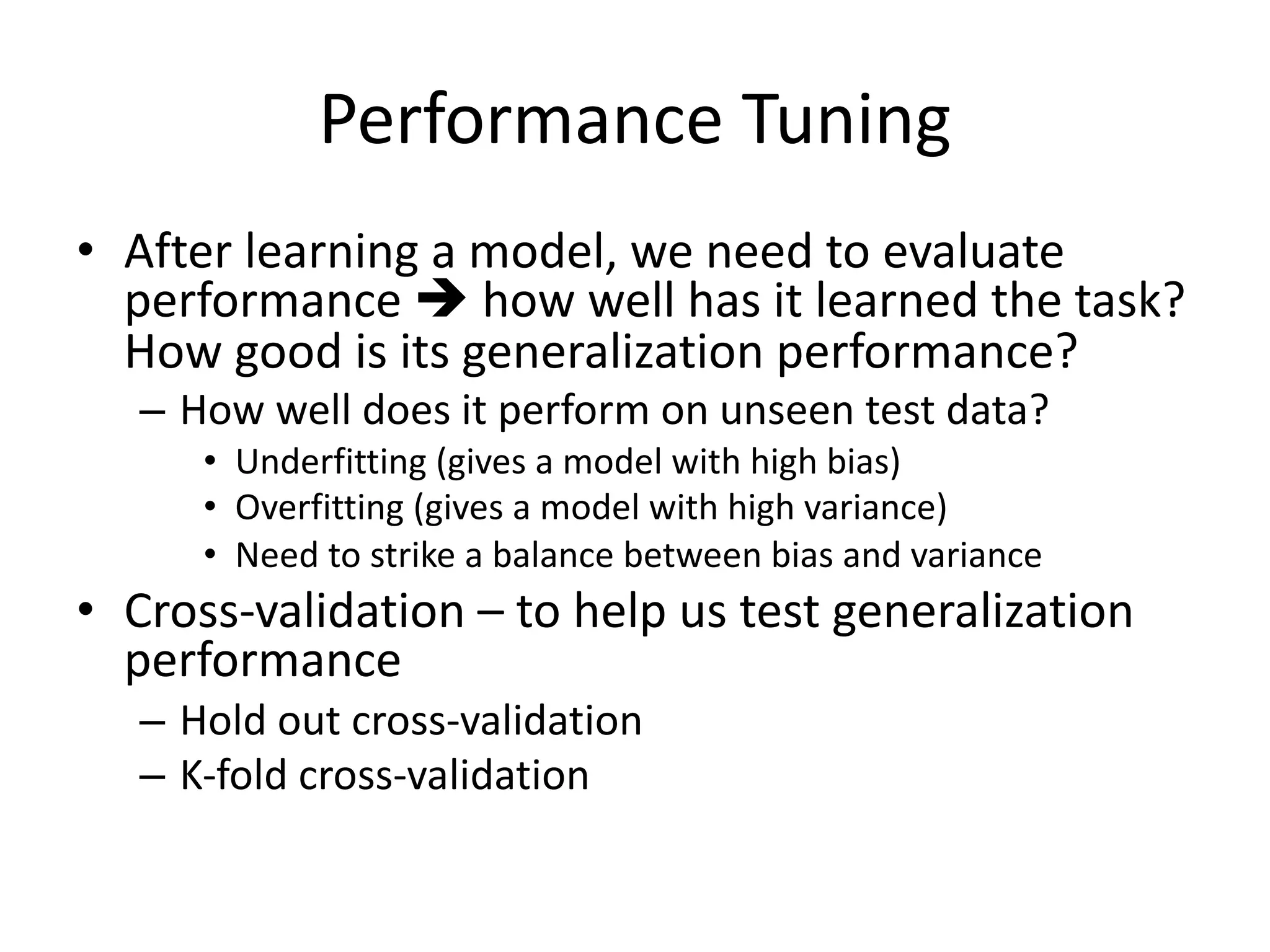
Performance Evaluation • After learning a model, we need to evaluate performance è how well has it learned the task? How good is its generalization performance? – How well does it perform on unseen test data? • How do we evaluate regression models? – Residual plot (residual errors vs. predicted values); residual errors expected to be randomly distributed and scattered around the center (y=0) line – MSE • Compare MSE for training vs. test data • Can be used to compare different regression models • Can be used to tune a given model’s hyper-parameters via grid search and cross-validation (if applicable to model structure) – Co-efficient of Determination (R2): • [0-1]; • gives the percentage variation in y explained by x-variables. A higher coefficient is an indicator of a better goodness of fit for the observations; Measure indicates the likelihood of unseen test data falling within the regression line.

Performance Tuning • After learning a model, we need to evaluate performance è how well has it learned the task? How good is its generalization performance? – How well does it perform on unseen test data? • Underfitting (gives a model with high bias) • Overfitting (gives a model with high variance) • Need to strike a balance between bias and variance • Cross-validation – to help us test generalization performance – Hold out cross-validation – K-fold cross-validation

Preprocessing • Raw data rarely in a shape/form that is necessary for optimal performance of ML algorithms – Preprocessing data thus a crucial first step! • Ensure features selected are on same scale for optimal performance of ML algorithm – Transform features into [0,1] range - normalization – Transform features to attain standard normal distribution with zero mean and unit variance • Dimensionality reduction needed if there’s high correlation between features making them redundant – Improves Signal to Noise ratio (SNR) – Reduces memory requirements – Faster run times for algorithm

References 1. Python Machine Learning: Machine Learning and Deep Learning with Python, scikit-learn, and TensorFlow 2; 3rd Edition; (2019) by Sebastian Raschka and Vahid Mirjalili 2. Evaluation of Regression Models: Model Assessment, Model Selection and Generalization Error by Frank Emmert-Streib et. al

Lecture 5 - Linear Regression Linear Regression

More Related Content

Similar to Lecture 5 - Linear Regression Linear Regression

Recently uploaded

Lecture 5 - Linear Regression Linear Regression