![Bias • Bias is defined as, Bias[f(X)] = E[ 𝐘] – Y • Bias can be reduced by, • Using a better ML algorithm • Using a larger model (i.e. with more parameters) • Training for more iterations if training was stopped earlier • Using a larger training data set • Reducing regularization (if exists) • Example for high bias, • Using a straight line to model a quadratic polynomial distribution](https://image.slidesharecdn.com/lec7-240412205954-6f933db6/75/Lecture-7-Bias-Variance-and-Regularization-a-lecture-in-subject-module-Statistical-Machine-Learning-10-2048.jpg)
![Variance • Variance is defined as, Variance[f(X)] = E[ {E( 𝐘)– 𝐘}2 ] • Variance can be reduced by • Using a larger training dataset can reduce the variance as the errors get cancelled out • Reducing the number of parameters can also reduce variance as the less significant insights (like noise) will not be included in the model • Can use Dimensionality Reduction and Feature Selection (will be discussed in future) • Using Early Stopping to stop training at an optimal point • Dropout is used in Deep Learning models (not relevant to out subject module ☺) • Increasing (or introducing, if not at the moment) regularization • Example for high variance, • Using a 8 degree polynomial to model a linear distribution](https://image.slidesharecdn.com/lec7-240412205954-6f933db6/75/Lecture-7-Bias-Variance-and-Regularization-a-lecture-in-subject-module-Statistical-Machine-Learning-12-2048.jpg)
![Error Composition • Mean Square Error, MSE{መ 𝐟 𝐱 } = [Bias{ 𝐘}]2 + Var{ 𝐘} • Error in prediction, E( 𝐘-Y)2 = MSE{መ 𝐟 𝒙 } + 𝝈 Where 𝝈 is the irreducible error Source: https://www.geeksforgeeks.org/bias-vs-variance-in-machine-learning/](https://image.slidesharecdn.com/lec7-240412205954-6f933db6/75/Lecture-7-Bias-Variance-and-Regularization-a-lecture-in-subject-module-Statistical-Machine-Learning-13-2048.jpg)
![Elastic Net Regression • Both L1 and L2 functionalities can be used by weighting each of its values, which results Elastic Net Regression • This will bring some small parameters to zero (due to the L1 effect) and reduce some larger parameters (due to the L2 effect) • Select 𝜶 to adjust the balance of the effect between L1 and L2 Loss := Loss + 𝛼 ∗𝜆 * σ𝑖=1 𝑛 |𝛽𝑖| + (1-𝛼) ∗𝜆 *𝑗=1 𝑚 𝛽𝑗 2 Where 0 < 𝛼 < 1 Loss := Loss + 𝜆 * [𝛼 ∗ σ𝑖=1 𝑛 |𝛽𝑖| + (1-α) ∗ 𝑗=1 m 𝛽𝑗 2 ]](https://image.slidesharecdn.com/lec7-240412205954-6f933db6/75/Lecture-7-Bias-Variance-and-Regularization-a-lecture-in-subject-module-Statistical-Machine-Learning-20-2048.jpg)


The document covers key concepts in machine learning, including model training, bias, variance, and regularization techniques. It discusses how bias occurs when a model is too simple, leading to underfitting, while variance arises from a model being overly complex, leading to overfitting. The document also explains the bias-variance tradeoff and introduces regularization methods like L1 and L2 to manage these issues in model performance.
Introduction to DA 5230 focusing on Statistical & Machine Learning. Overview by Maninda Edirisooriya.
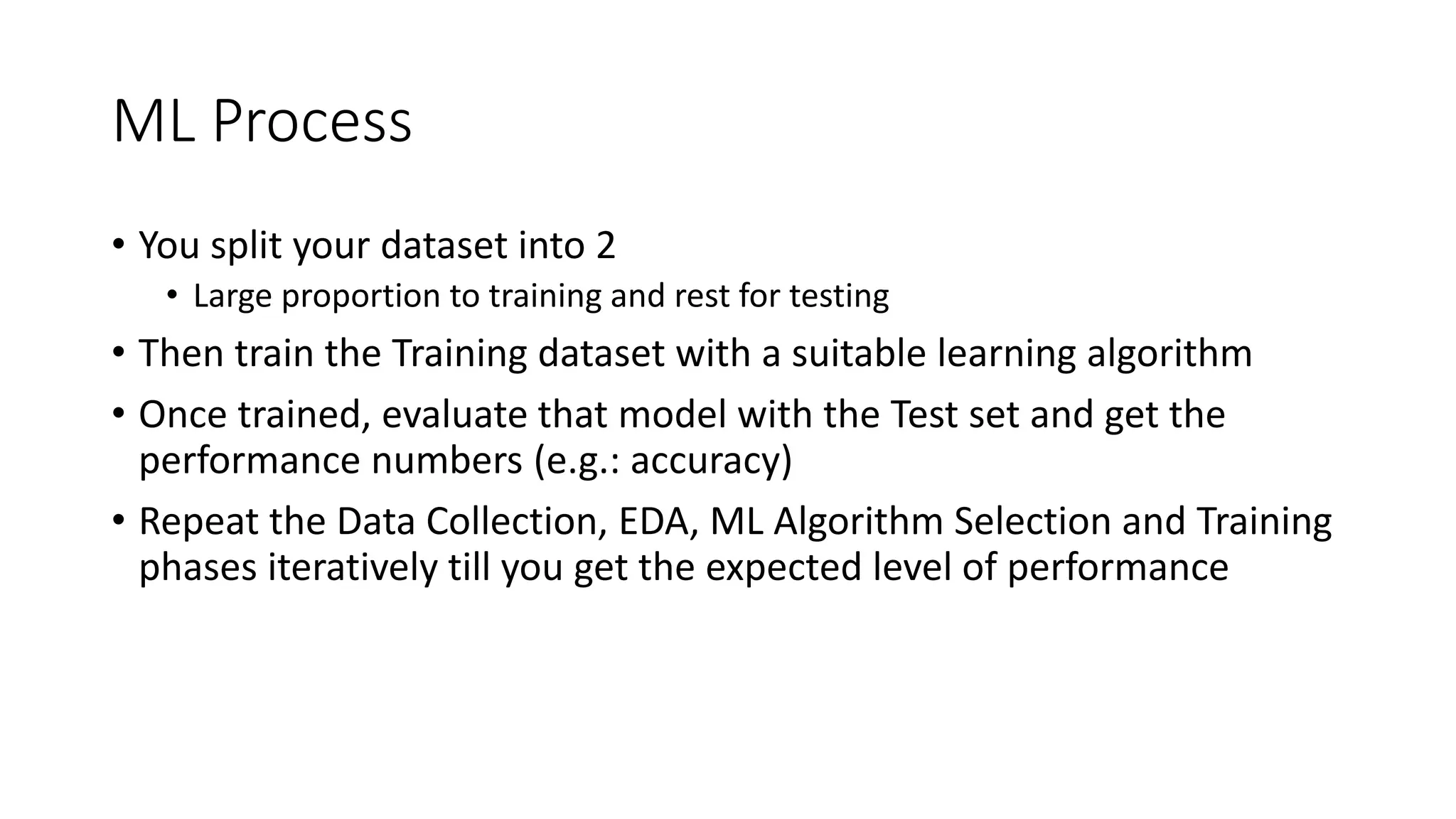
Description of the ML process involving dataset splitting, training, testing, and model evaluation iterations.
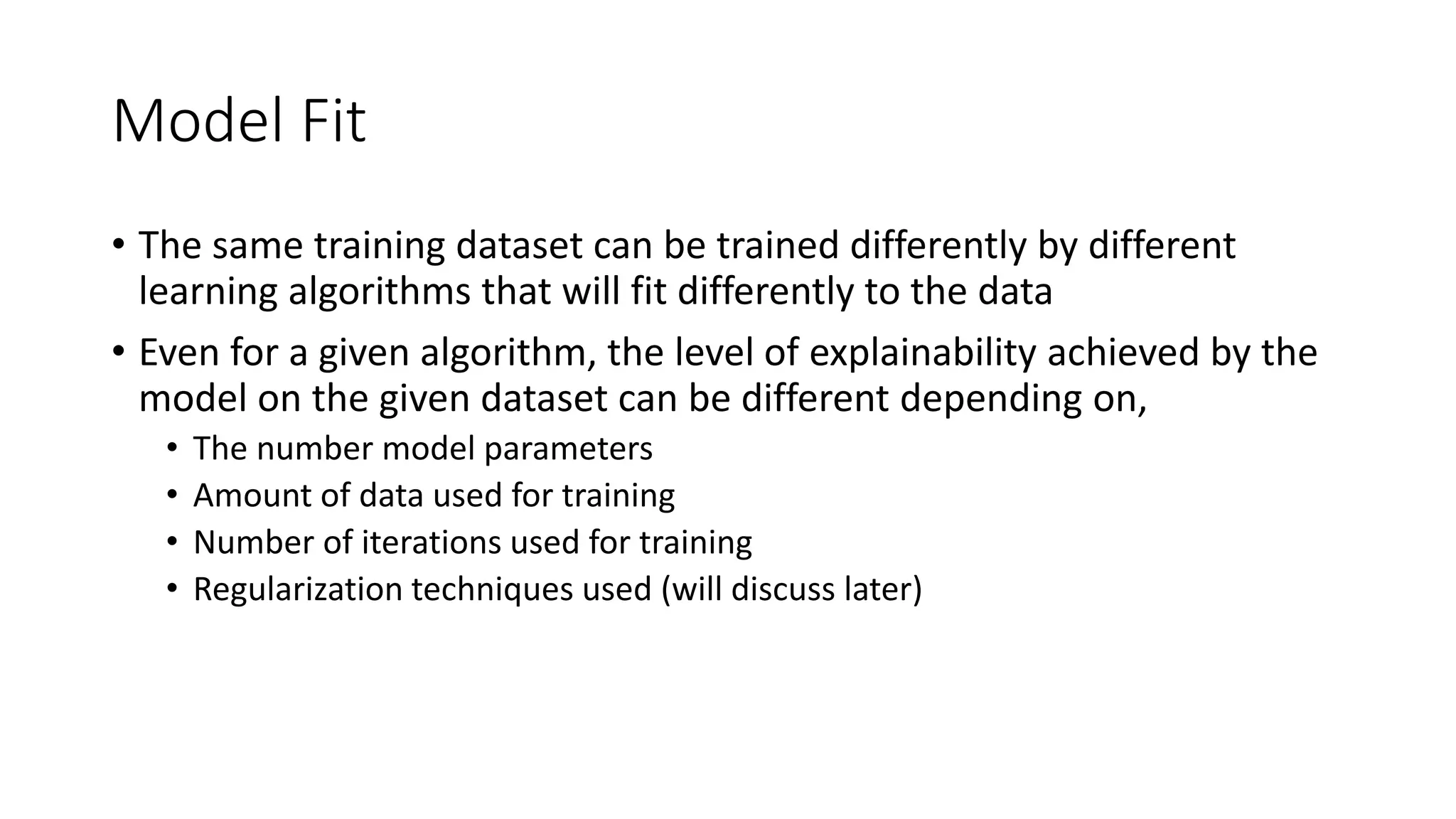
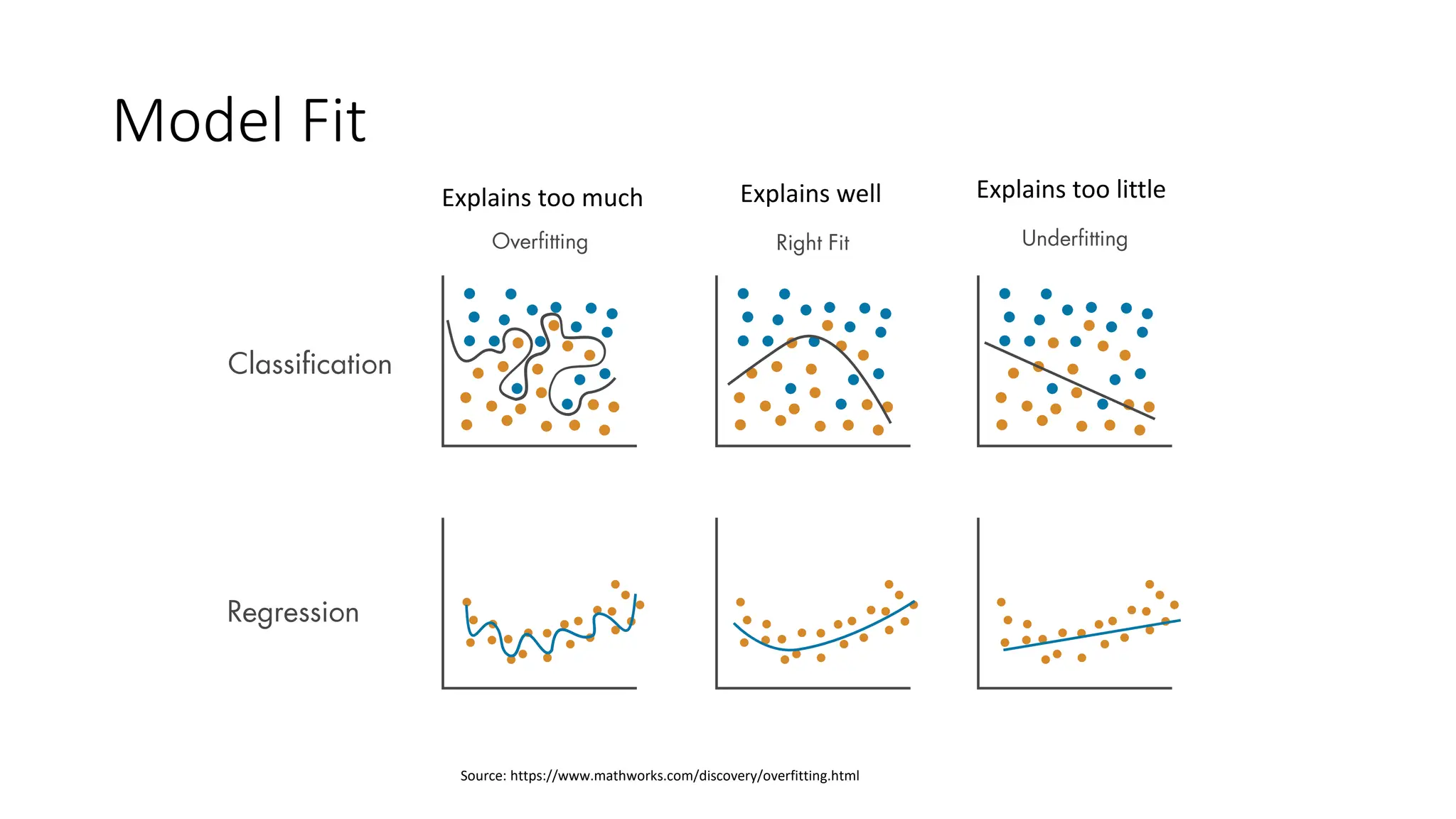
Explains how different algorithms can fit the same training dataset variably and the implications of different model fits.
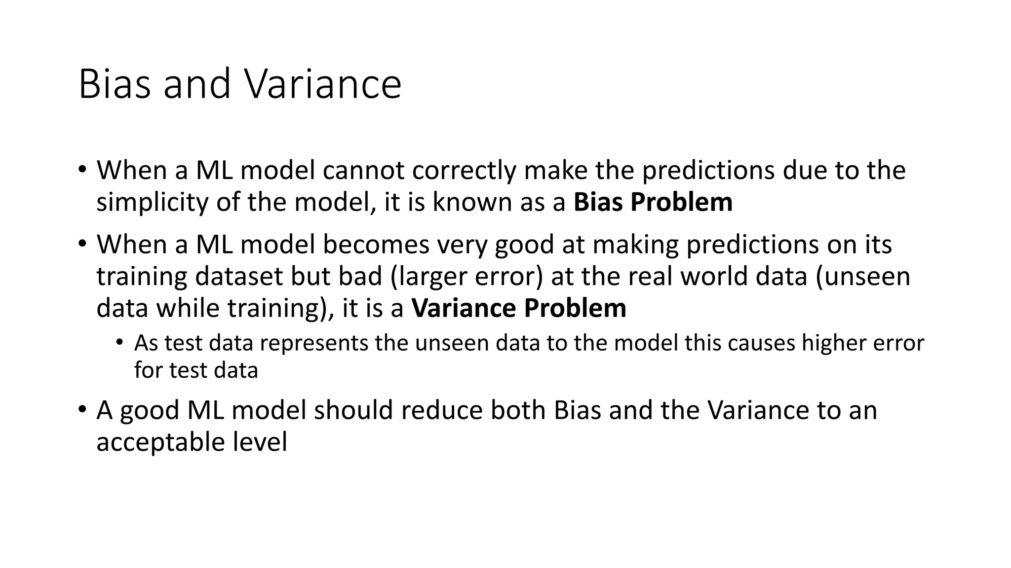
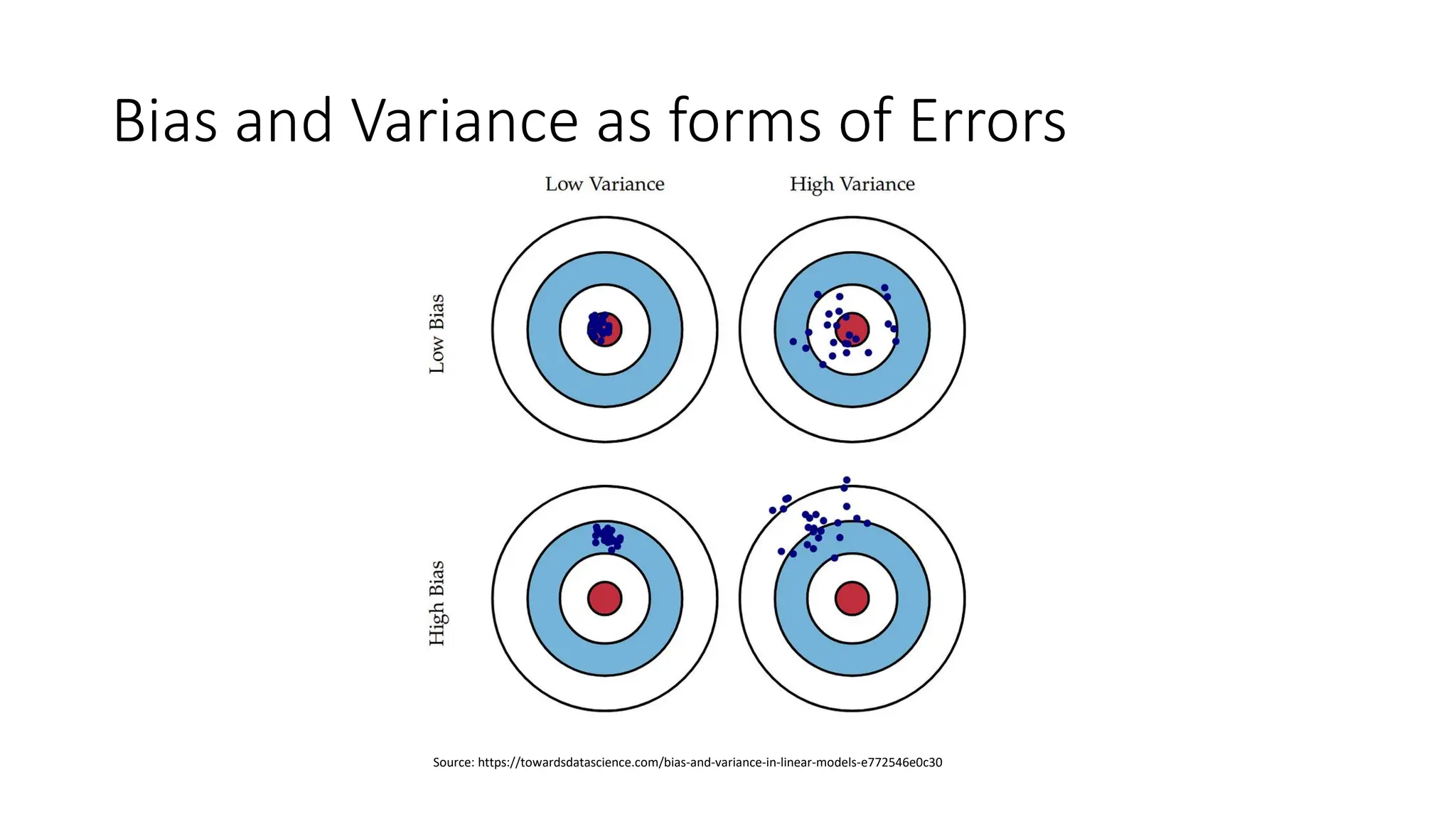
Definitions of Bias and Variance in ML, explaining their effects on model predictions and testing accuracy.
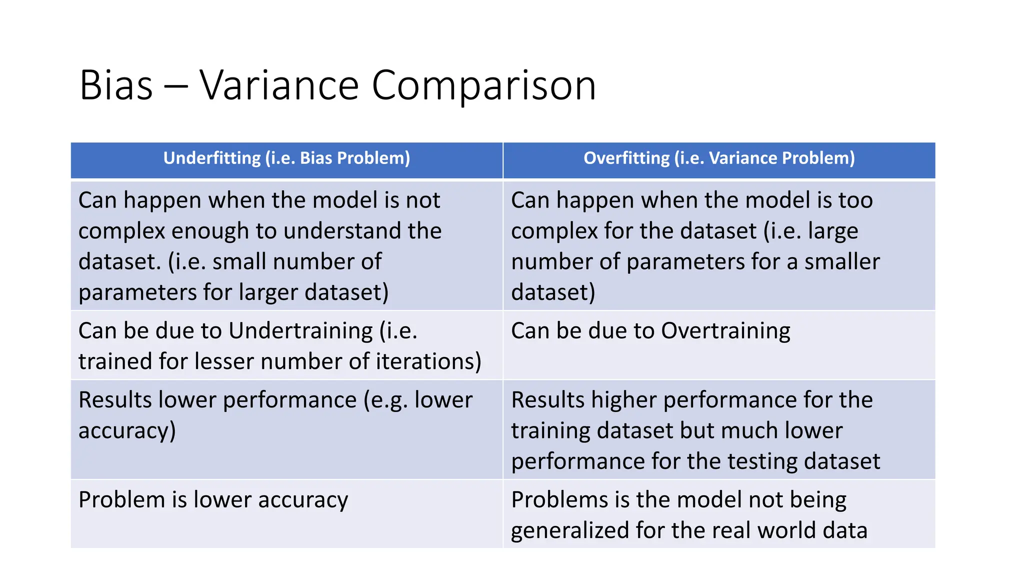
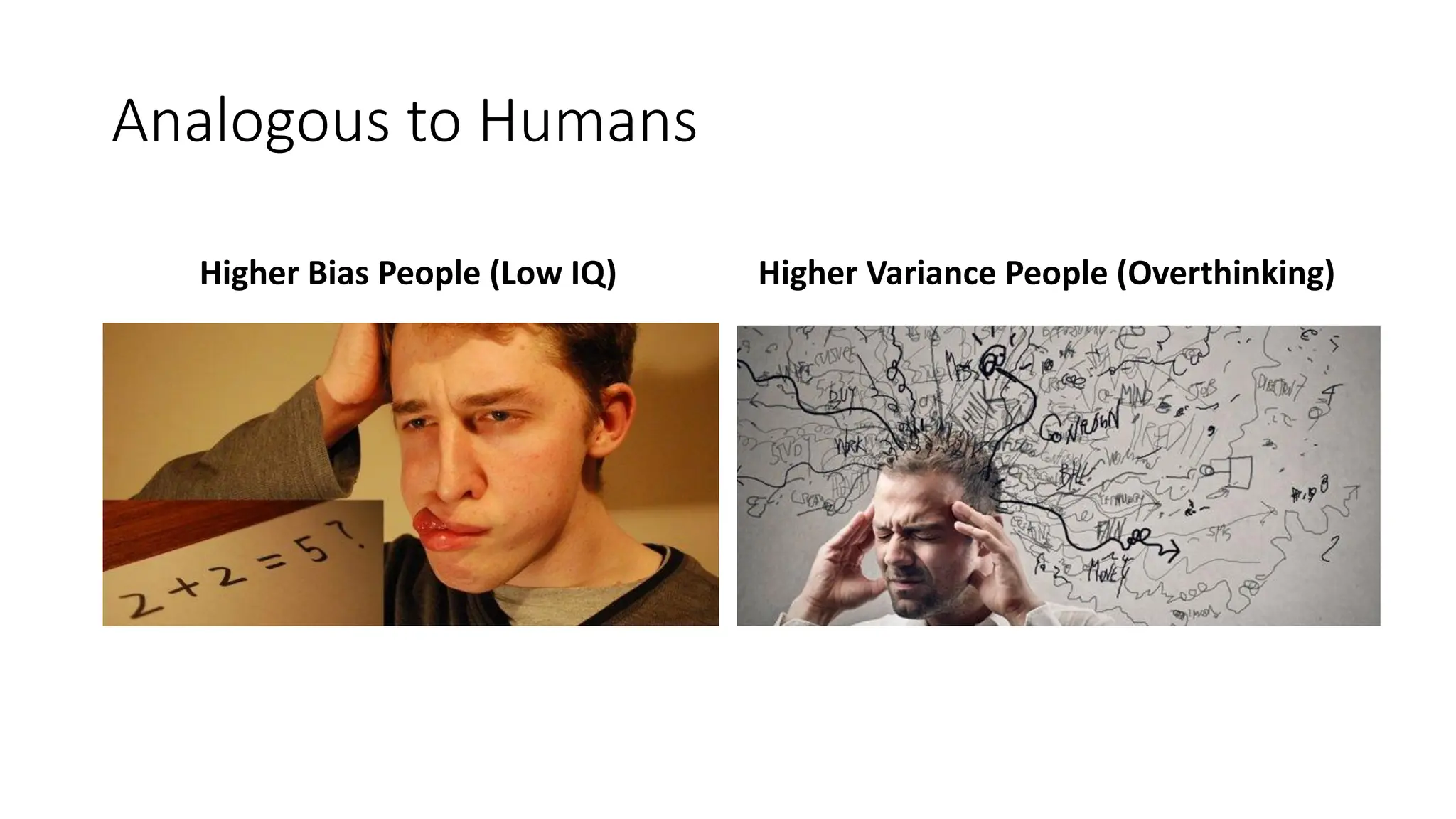
Comparison of underfitting (bias) and overfitting (variance) with analogies to human behavior for better understanding.
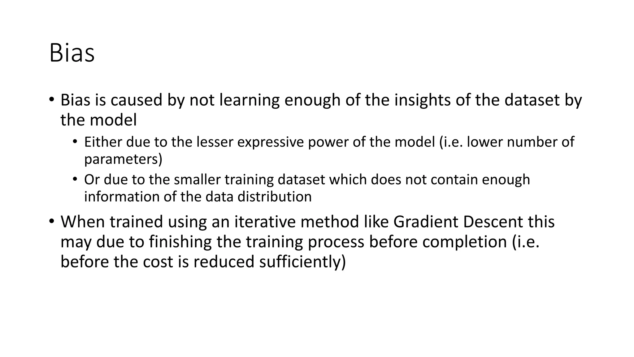
In-depth discussion on Bias, causes, reduction strategies, and an example illustrating its effects on modeling.
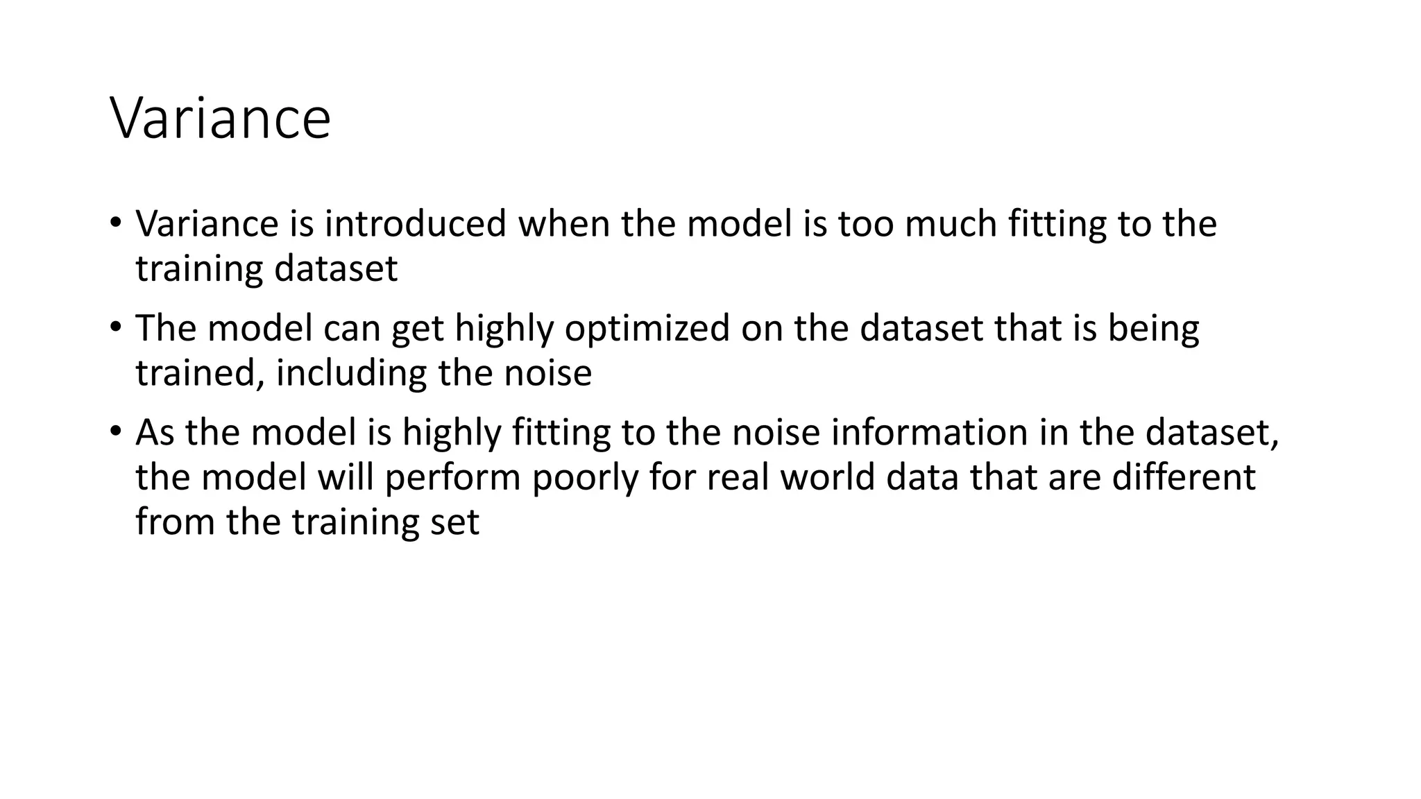
Explanation of Variance, its causes, methods of reduction, and an example demonstrating high variance issues.
Overview of Mean Square Error (MSE) composition linking bias, variance, and irreducible error.
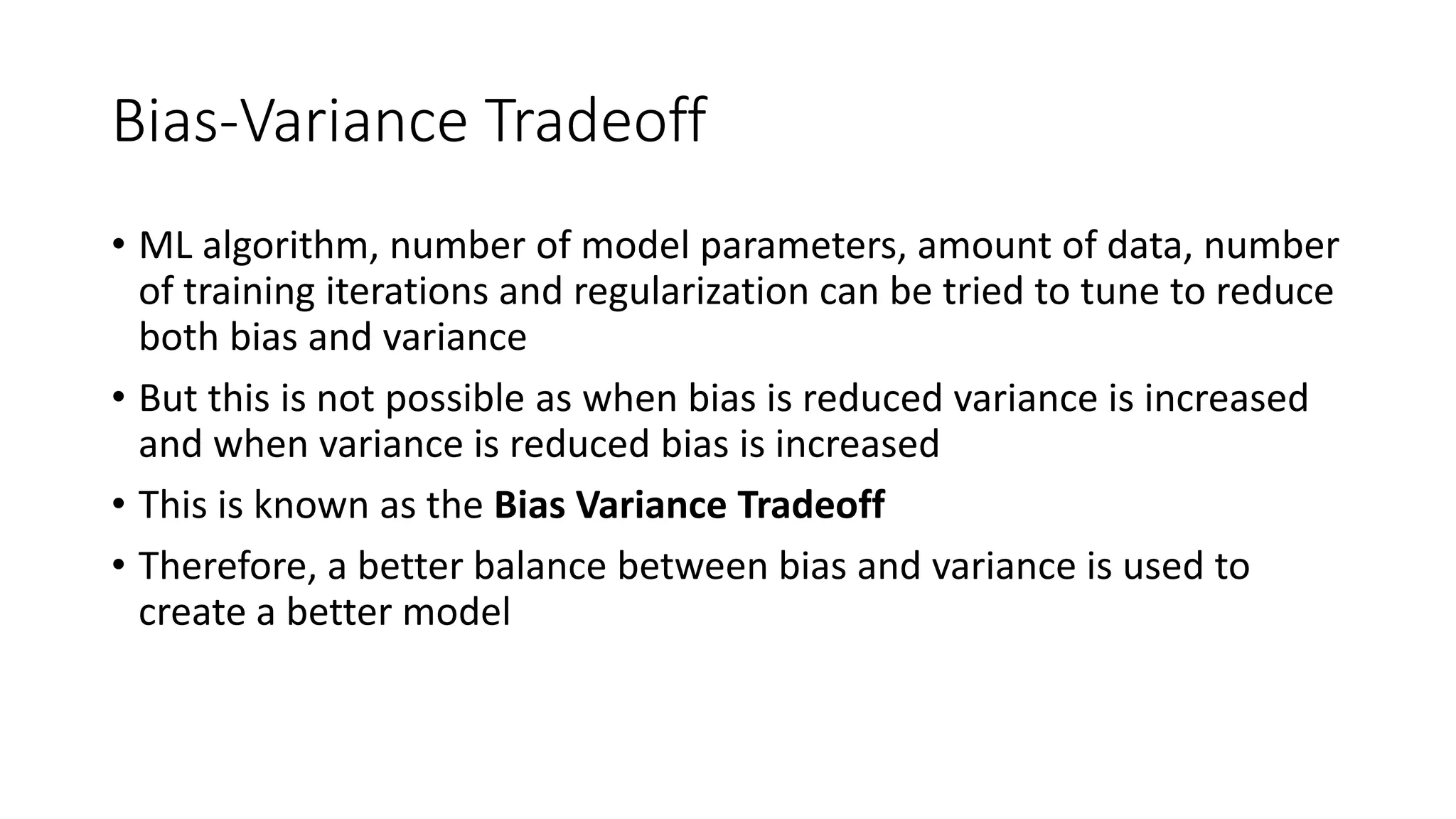
The concept of Bias-Variance Tradeoff, where reducing one leads to increasing the other, leading to balancing the two.
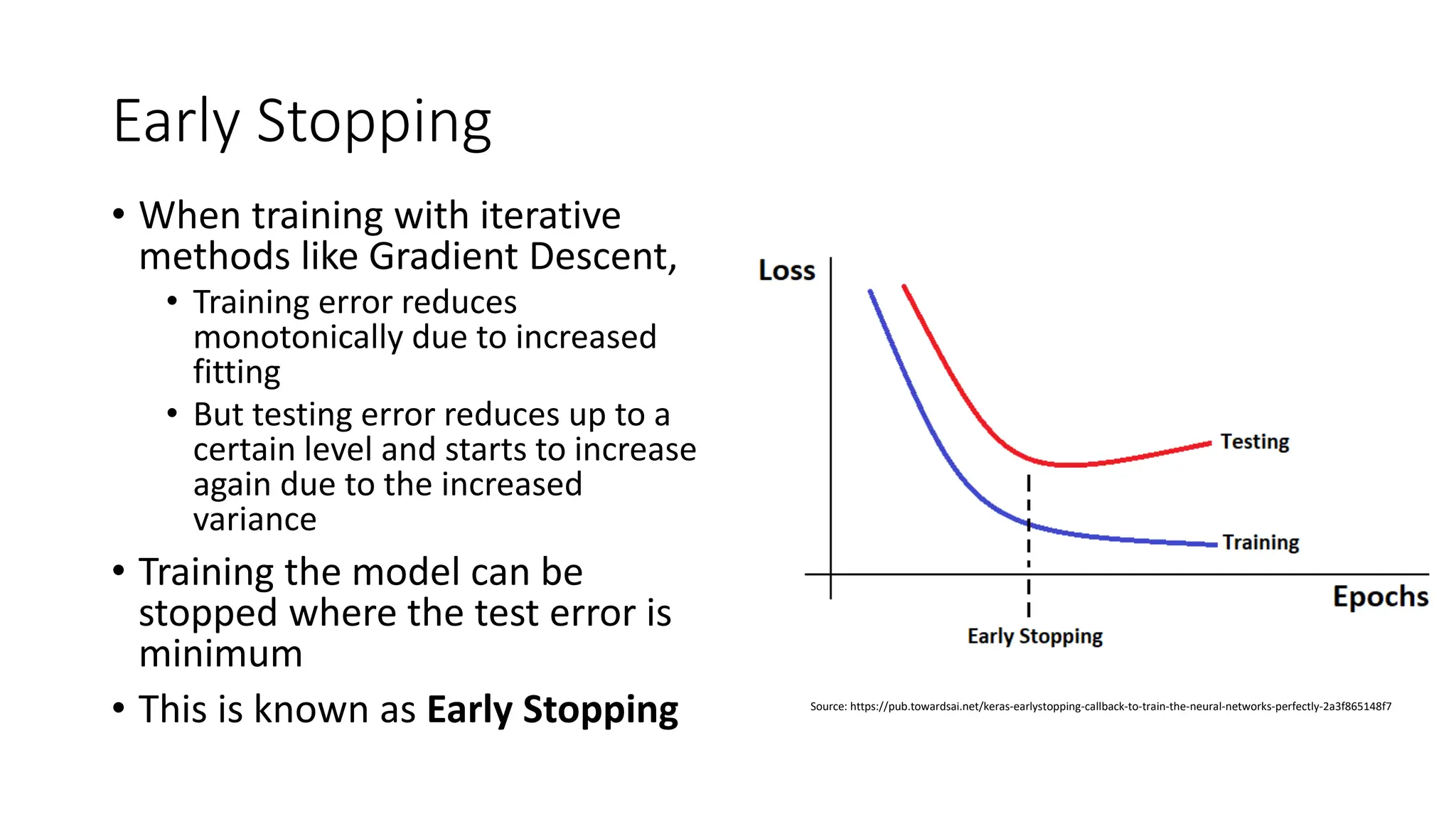
Explanation of Early Stopping in ML to halt training at optimal points to minimize testing error post certain fitting.
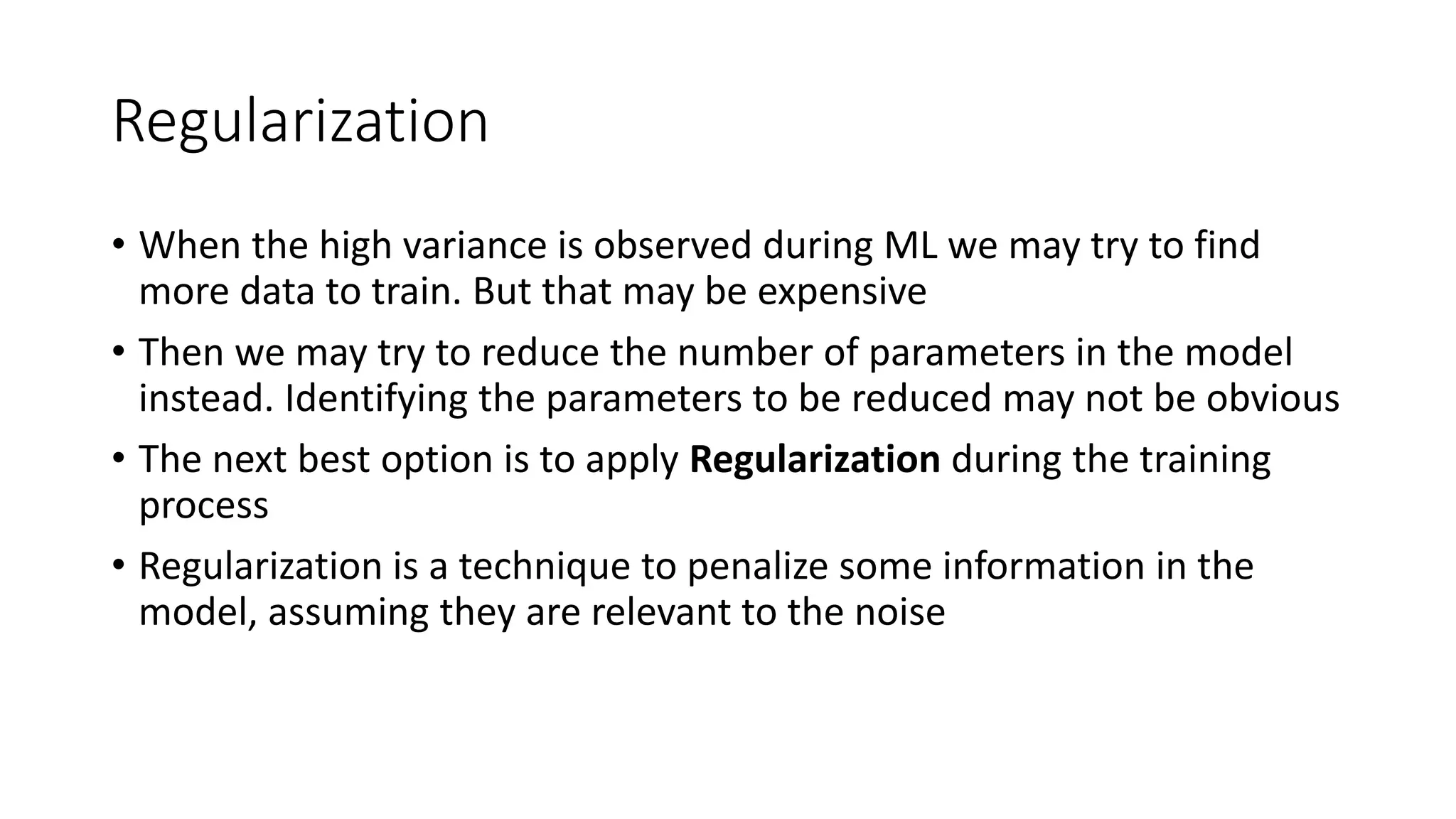
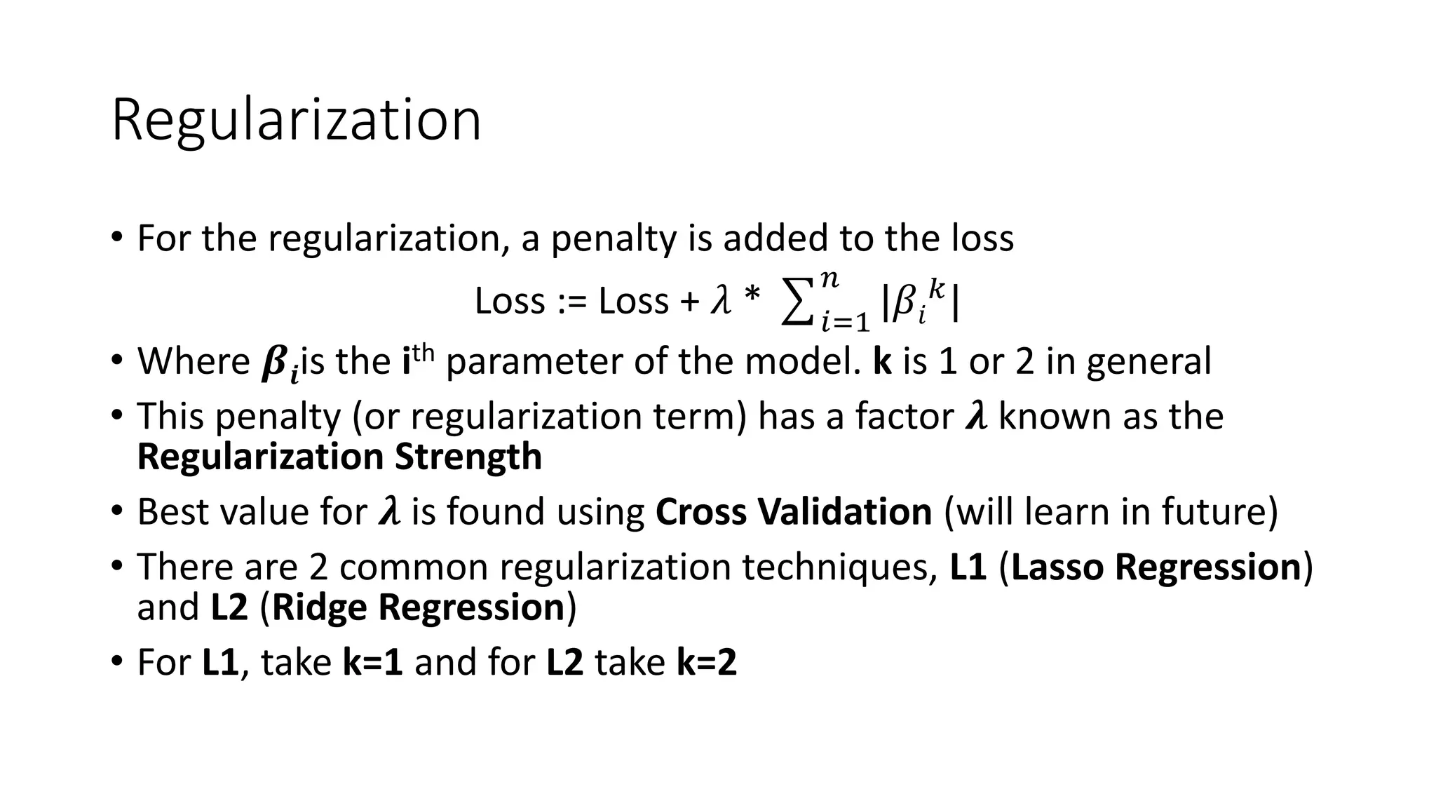
Introduction to Regularization, its purpose in reducing high variance, and penalties in loss functions for training models.
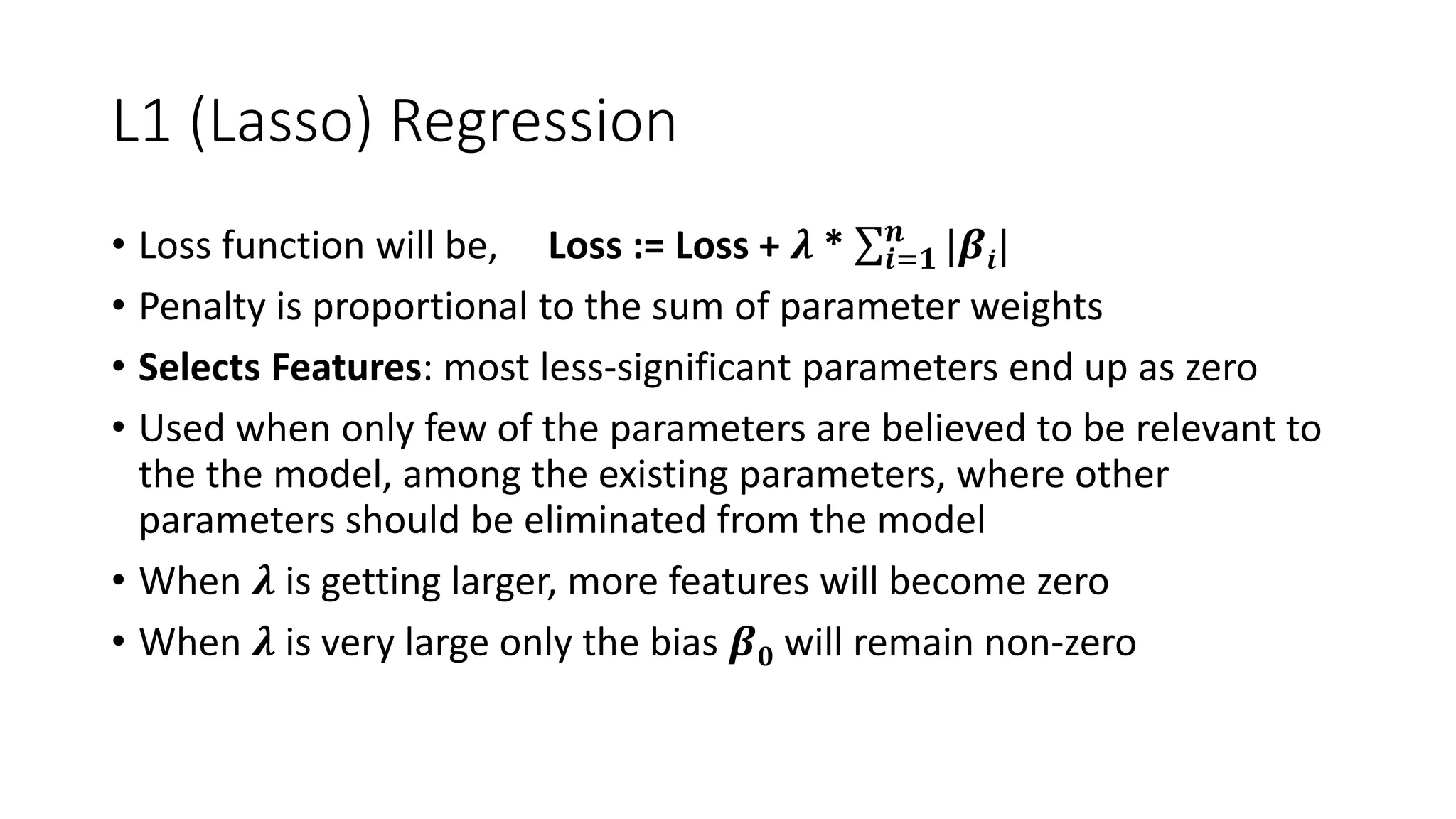
Detailed view of L1 (Lasso) regression, focusing on feature selection and its implications as regularization grows.
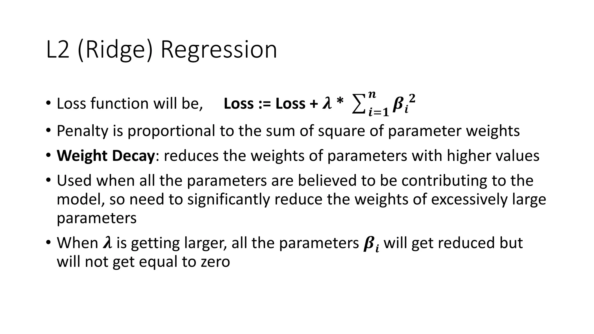
Detailed view of L2 (Ridge) regression, emphasizing weight decay and its effects on model parameters.
Introduction to Elastic Net Regression combining L1 and L2 techniques for feature selection and weight reduction.
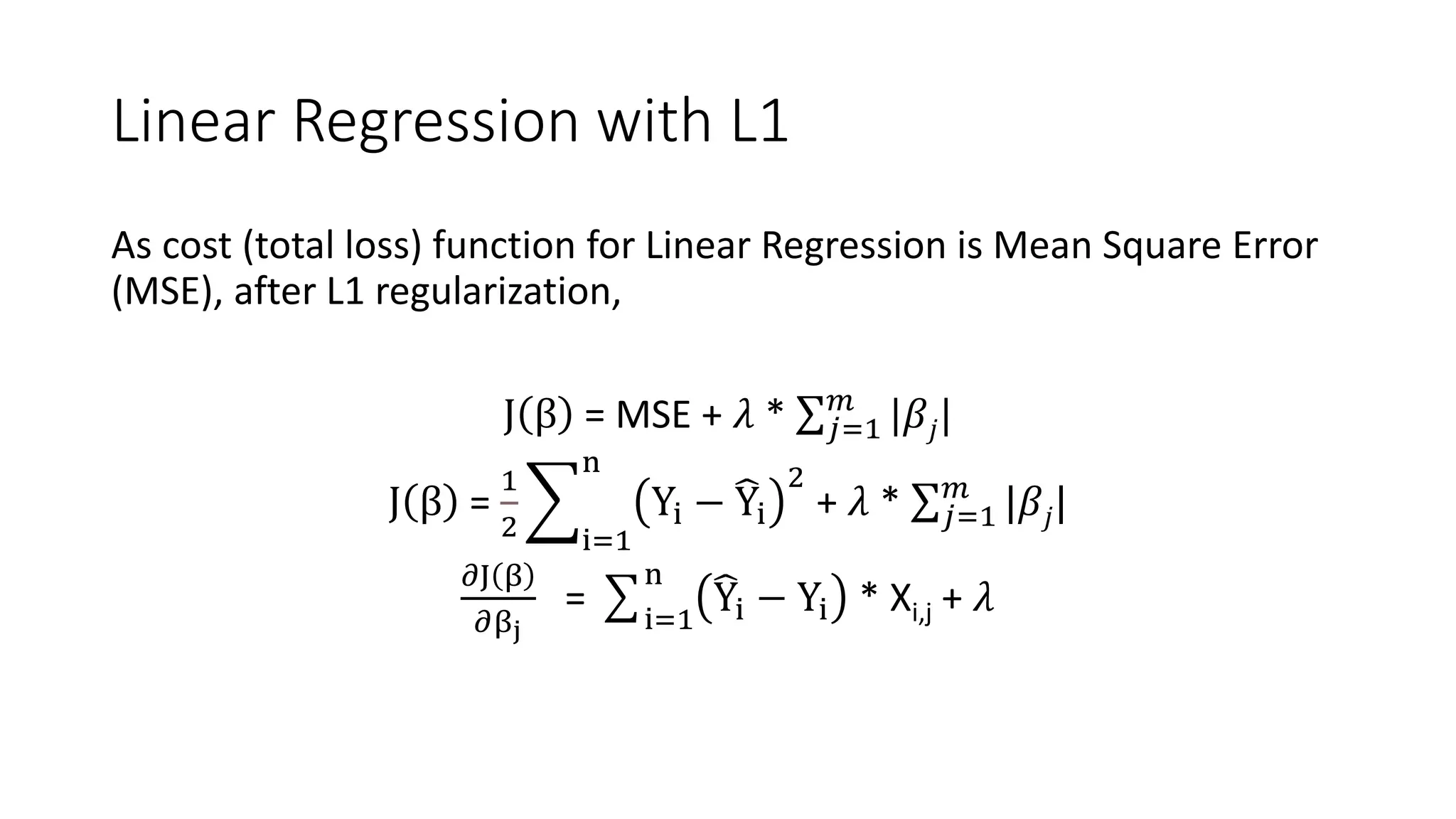
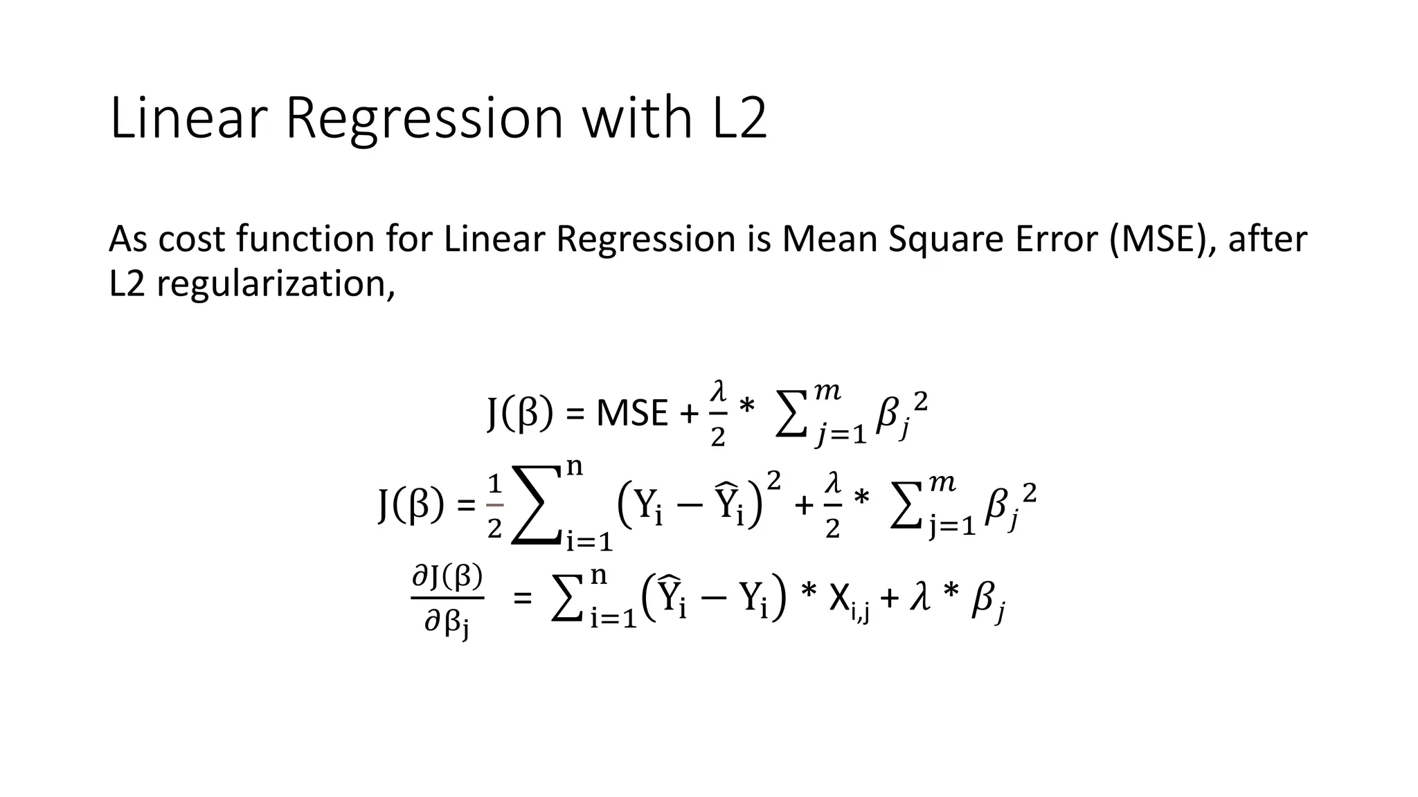
Exploration of cost functions for Linear Regression after applying L1 and L2 regularization with relevant formulas.
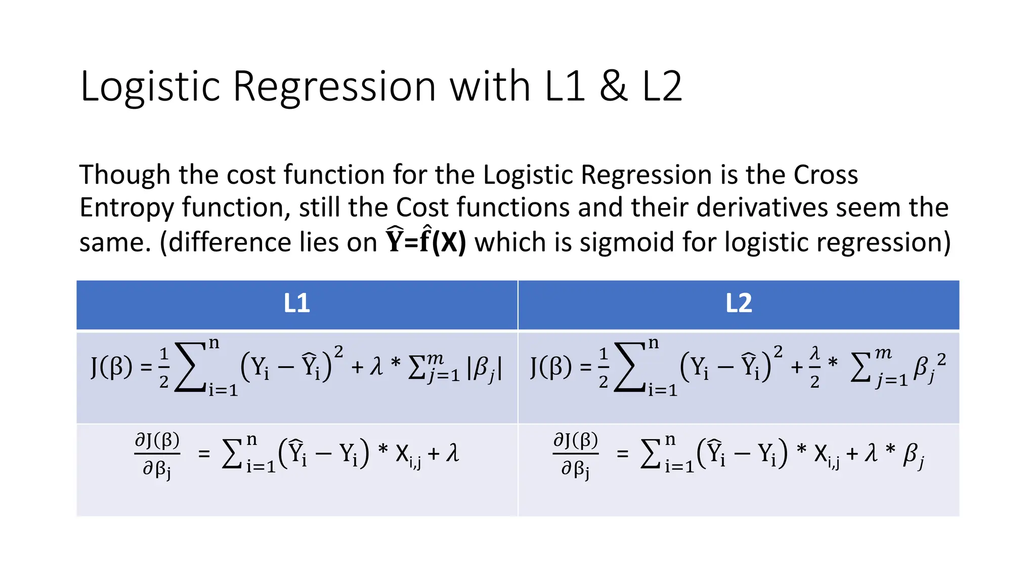
Description of cost functions and regularization techniques in Logistic Regression, drawing parallels with linear cases.
Assignment highlighting the importance of Bias, Variance, and Regularization in ML for further study.
Open floor for any questions regarding the lecture contents.