LOAD BALANCED CLUSTERING WITH MIMO UPLOADING TECHNIQUE FOR MOBILE DATA GATHERING IN WIRELESS SENSOR NETWORK
This project report details a proposed three-layer framework for mobile data collection in wireless sensor networks, utilizing distributed load balanced clustering and dual data uploading techniques, termed lbc-mimo. The framework aims to enhance scalability, extend network lifetime, and reduce data collection latency, with implementations demonstrating significant energy savings compared to traditional methods. The document includes comprehensive explanations of mobile computing concepts, system designs, implementation processes, and performance evaluations.
Project titled 'Load Balanced Clustering with MIMO Uploading Technique' submitted as part of M.Tech degree requirements and certification for project work completion.
Acknowledgments expressed for guidance, support, and infrastructure aid from various individuals and faculty that aided in project completion.
Comprehensive organization of the project document including chapters on Mobile Computing, Literature Review, Existing and Proposed Systems, Design, Implementation, Evaluation, and Conclusions.
An introduction to mobile computing, applications in various scenarios, and benefits including flexibility, productivity, and enhancement in business processes.
Discussion of WSNs, their structure, applications like monitoring and industrial use, characteristics, platforms, and concepts like data integration and in-network processing.
Overview of the current state of research in WSN data collection, energy consumption issues, and proposed new techniques for optimization.
Analysis of existing data collection methods, including relay routing and clustered systems, discussing their limitations in energy consumption and efficiency.
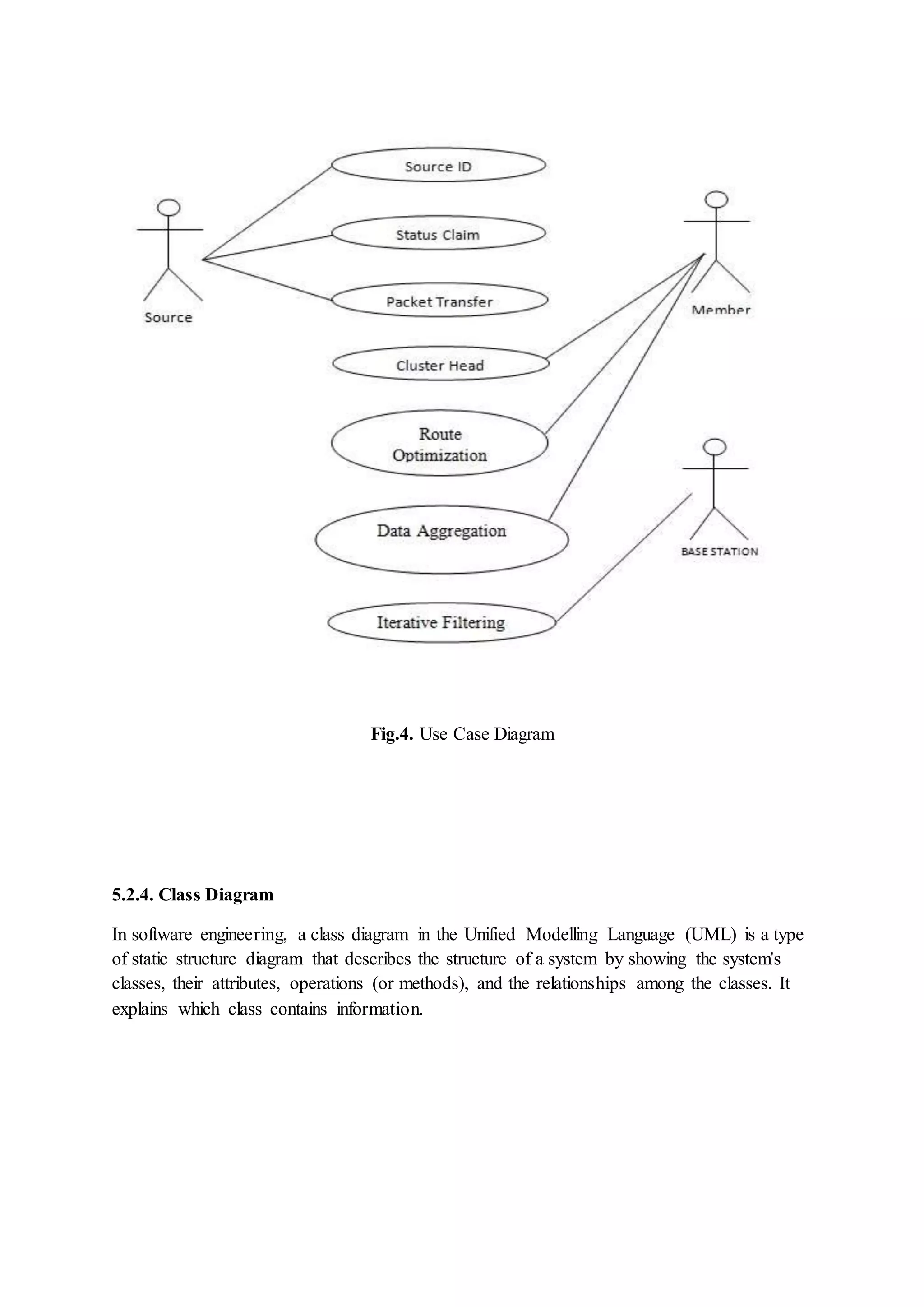
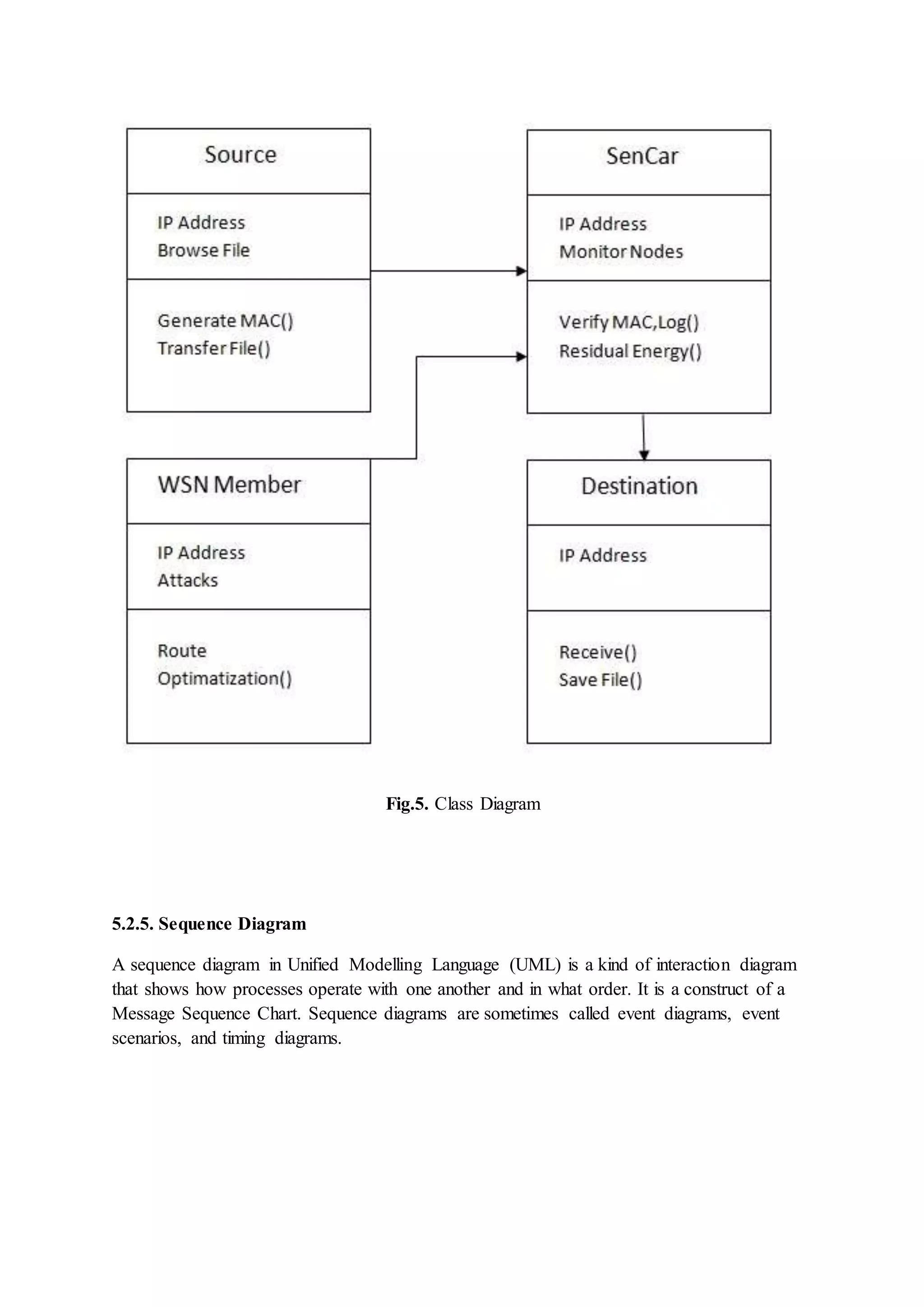
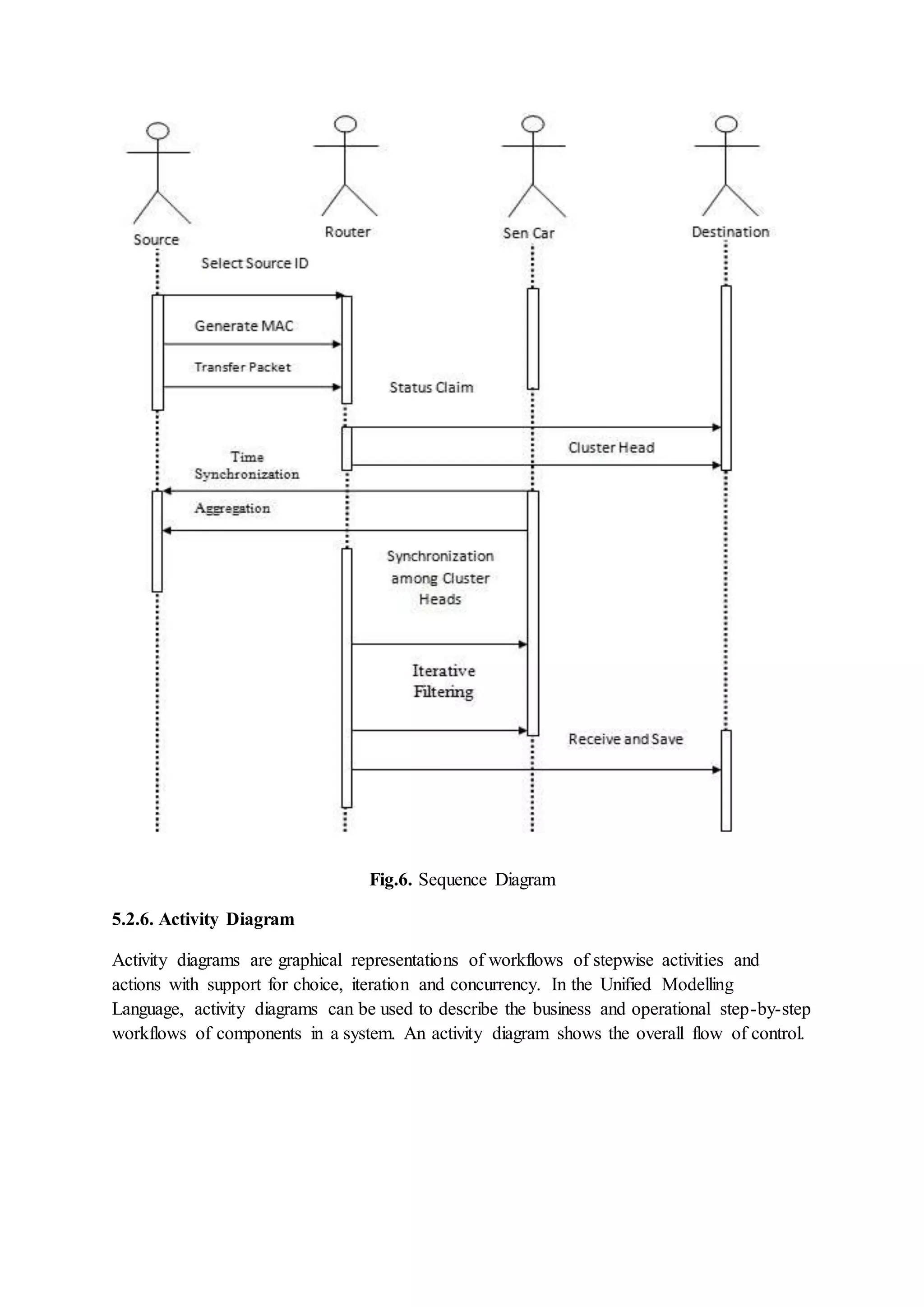
Introduction of the LBC-MIMO framework consisting of three layers focused on efficient mobile data collection, including specifics on clustering and communication methods.
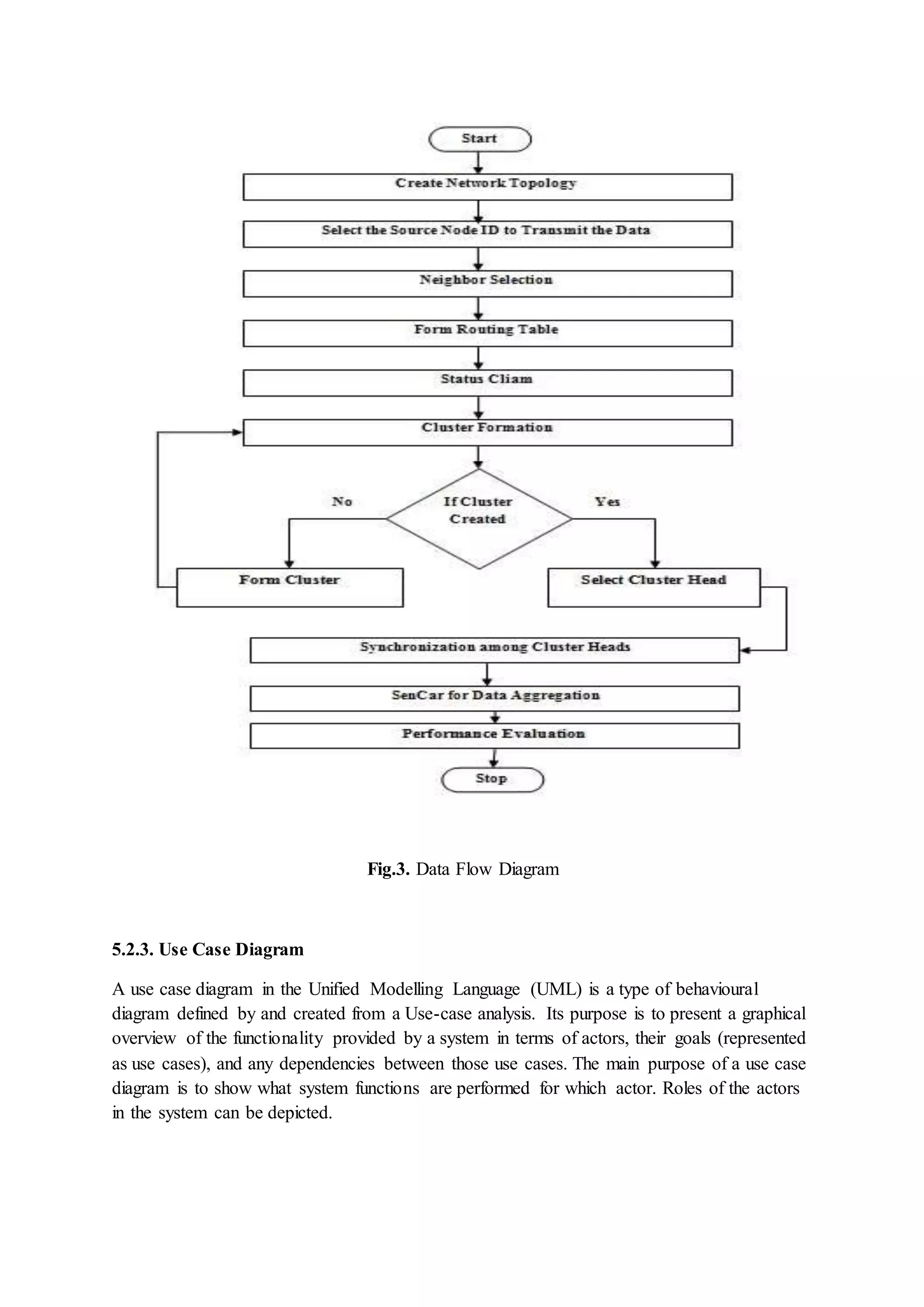
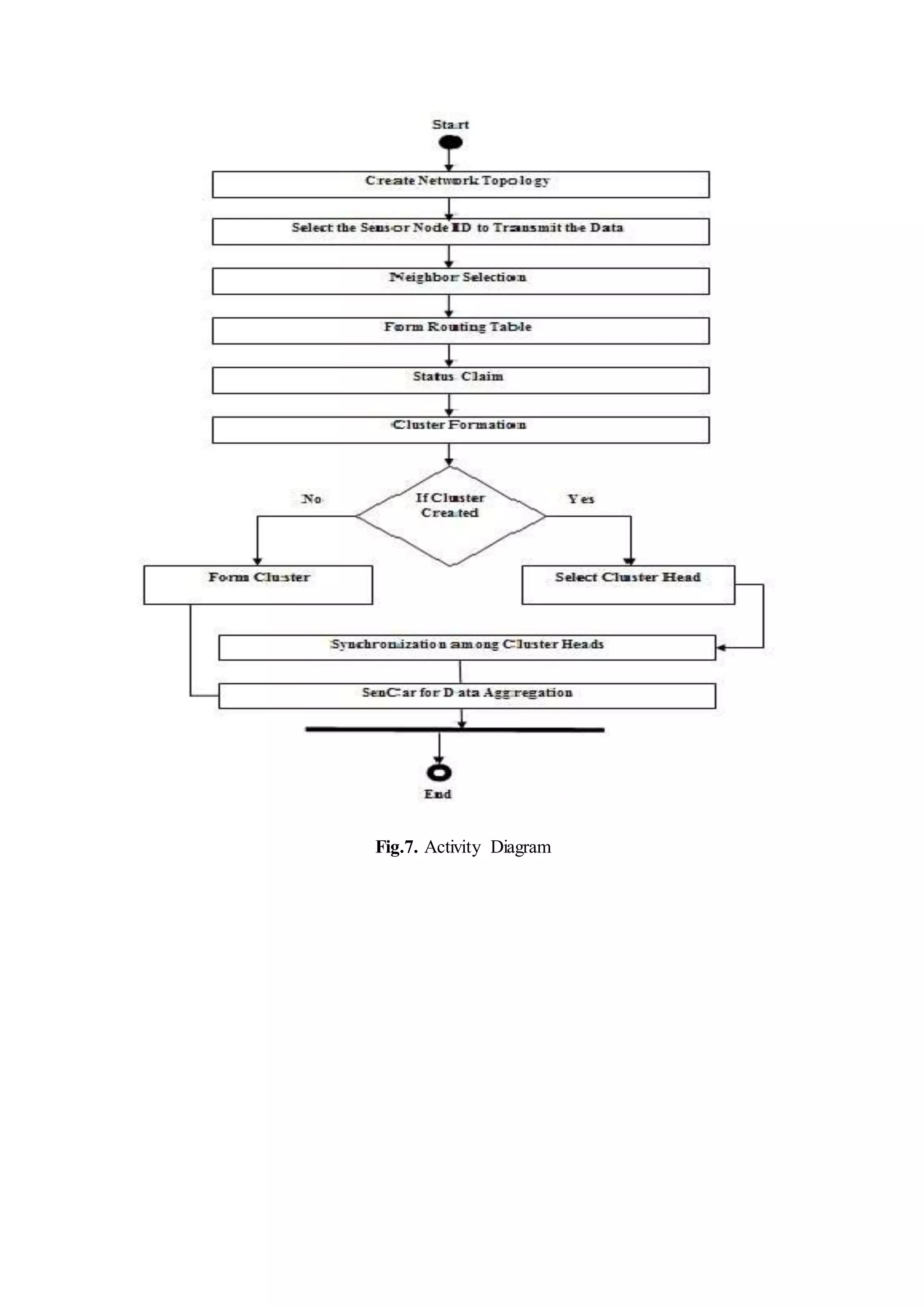
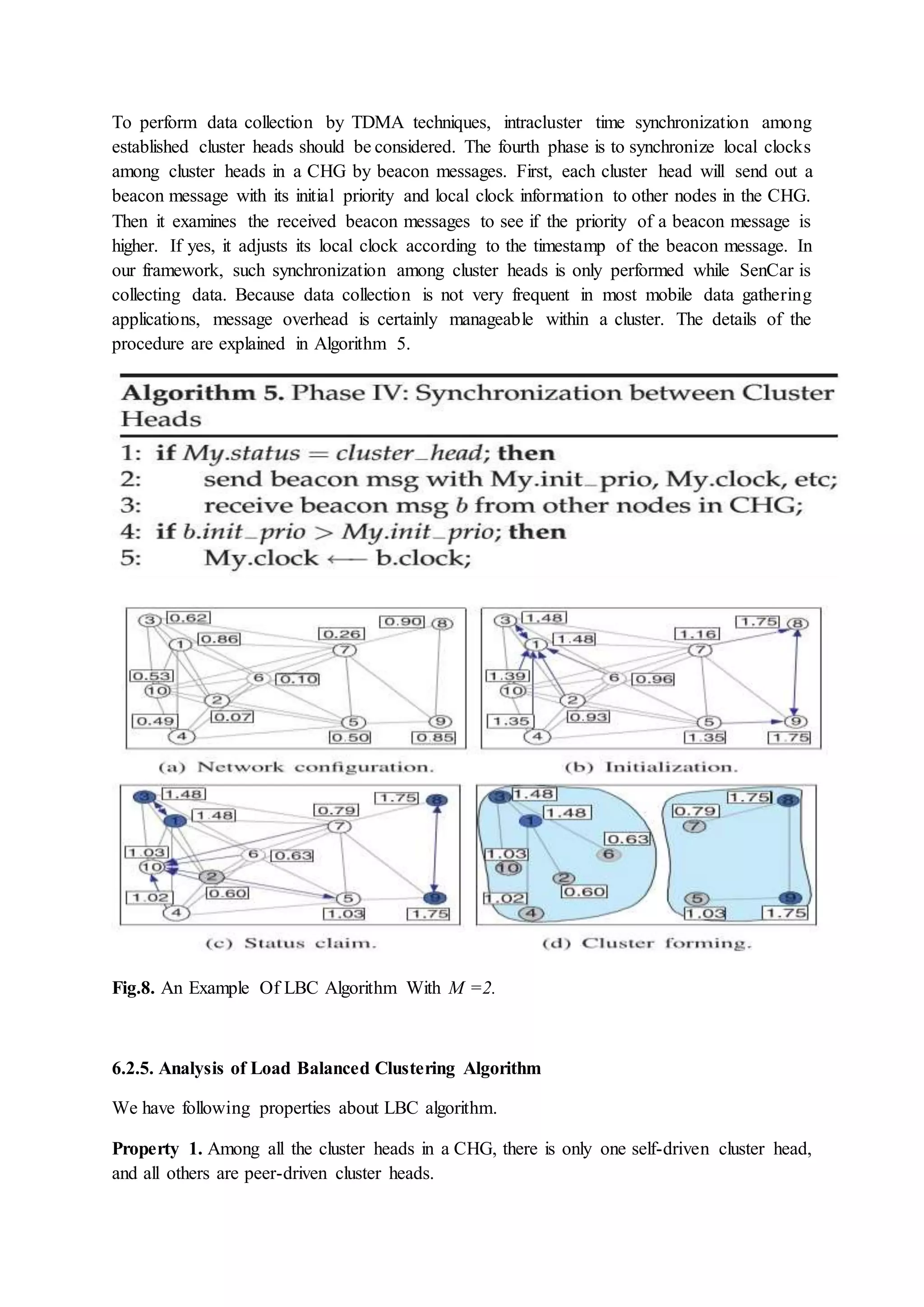
Detailed description of the implementation of the load balanced clustering algorithm, including initialization, status claims, clustering procedures, and synchronization.
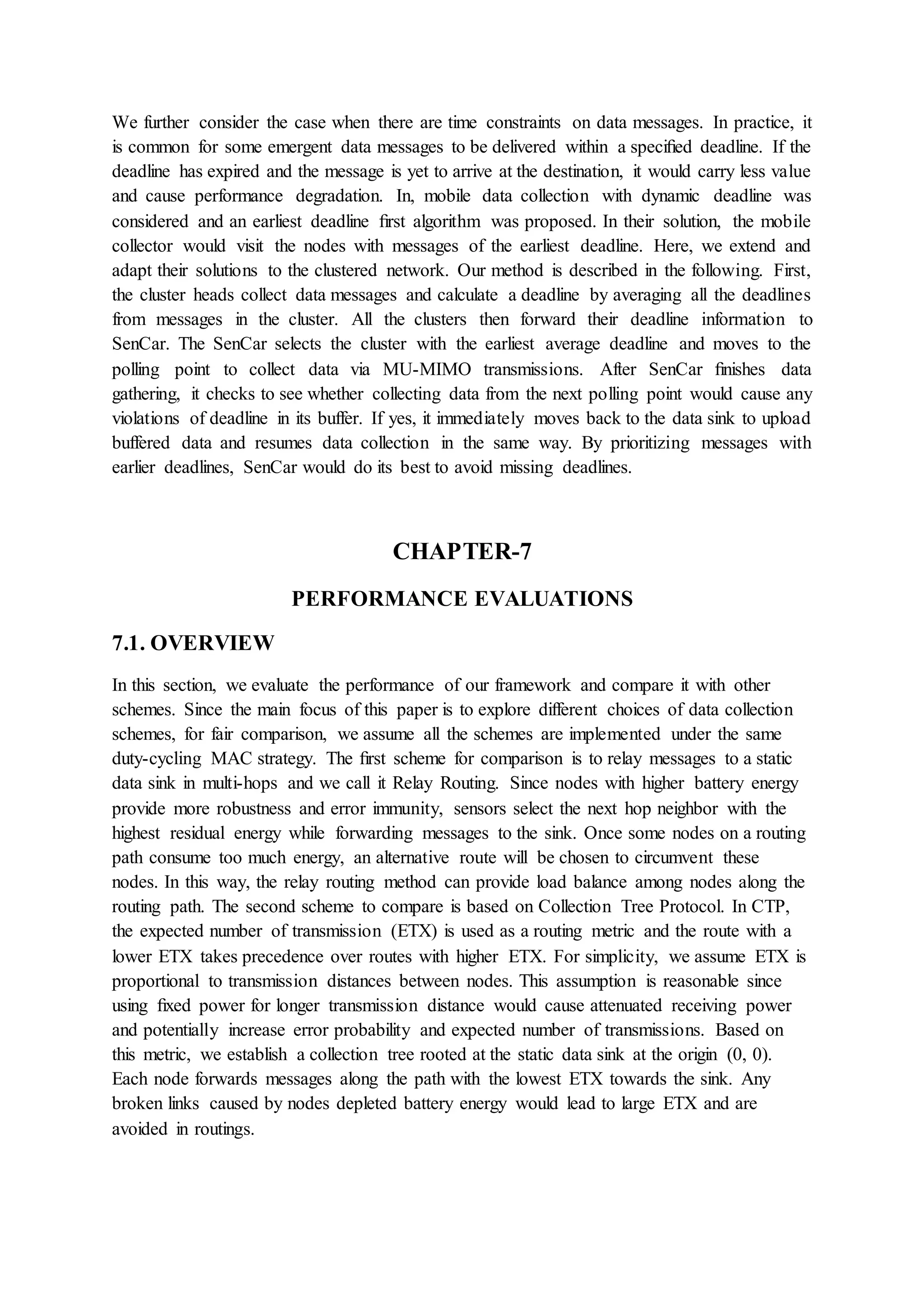
Evaluation of LBC-MIMO's performance including energy savings, data collection latency, effectiveness compared with existing methods, and load distribution among cluster heads.
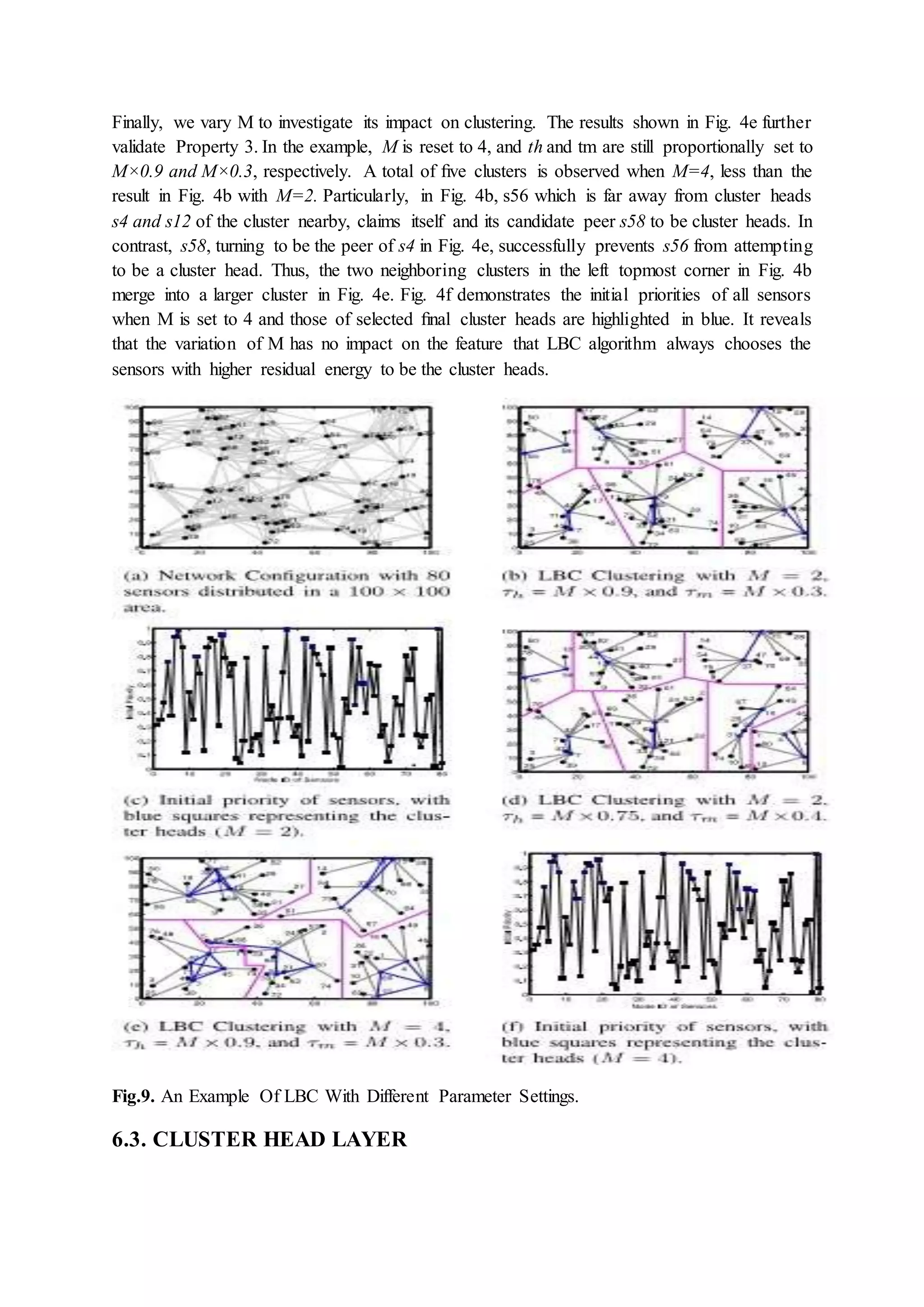
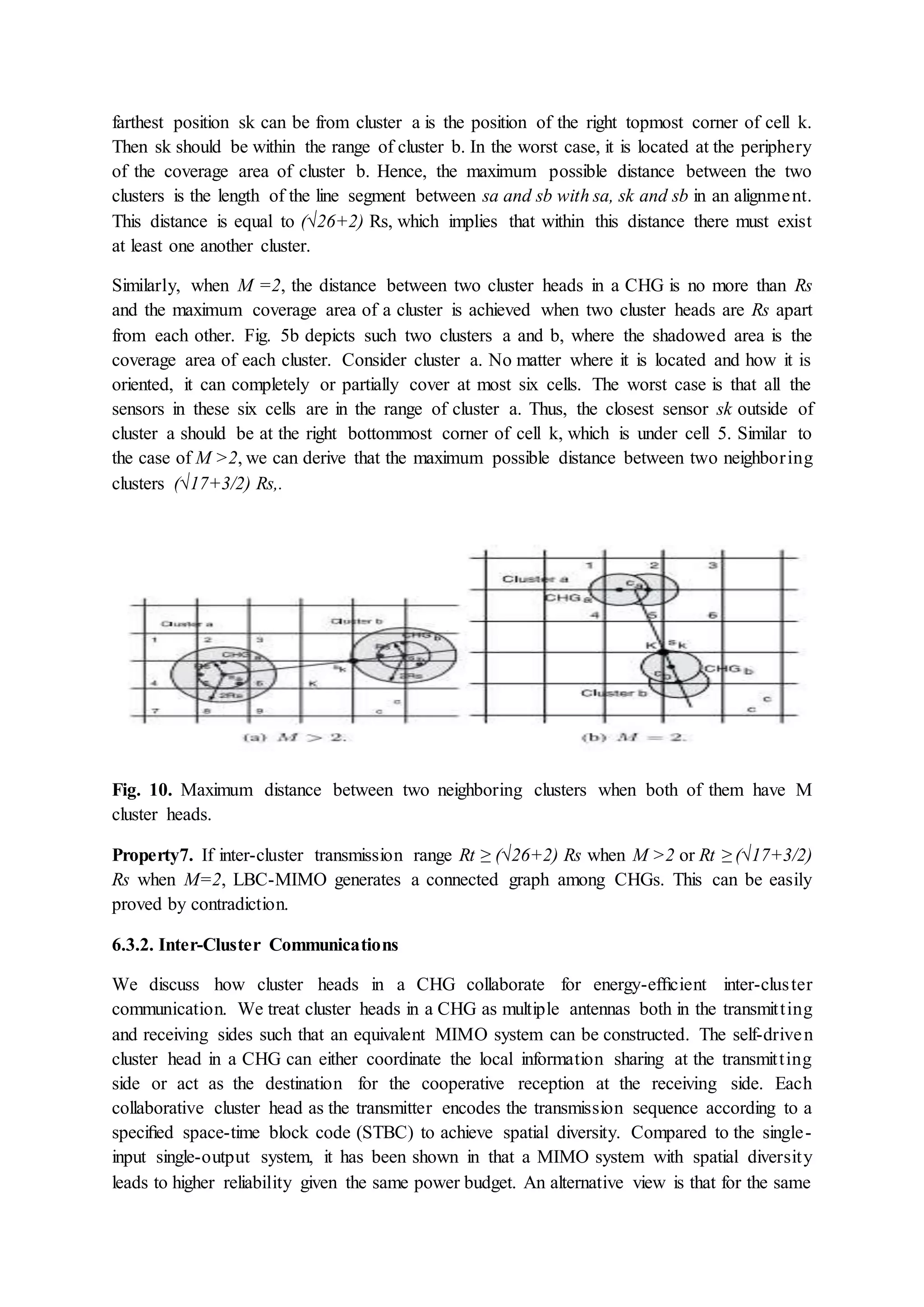
Concluding remarks on the LBC-MIMO framework's effectiveness and areas for future research, particularly in optimizing polling point selection and MIMO scheduling.
LOAD BALANCED CLUSTERING WITH MIMO UPLOADING TECHNIQUE FOR MOBILE DATA GATHERING IN WIRELESS SENSOR NETWORK
1.
LOAD BALANCED CLUSTERINGWITH MIMO UPLOADING TECHNIQUE FOR MOBILE DATA GATHERING IN WIRELESS SENSOR NETWORK A Project Report Submitted to JAWAHARLAL NEHRU TECHNOLOGICAL UNIVERSITY, ANANTAPURAMU By GUNAPATI.MUNISEKHAR (14KB1D5802) Under the esteemed Guidance Of Dr. S.MaruthuPerumal, M.E., Ph.D., Professor& Head, Dept. of C.S.E. Project report submitted in partial fulfillment of the Requirements for the award of the degree of MASTER OF TECHNOLOGY IN COMPUTER SCIENCE AND ENGINEERING DEPARTMENT OF COMPUTER SCIENCE AND ENGINEERING N.B.K.R INSTITUTE OF SCIENCE AND TECHNOLOGY (AN AUTONOMOUS INSTITUTION) VIDYANAGAR – 524 413 OCTOBER 2016
2.
Website: www.nbkrist.org. Ph:08624-228 247 Email : ist@nbkrist.org. Fax: 08624-228 257. N.B.K.R. INSTITUTE OF SCIENCE & TECHNOLOGY AUTONOMOUS INSTITUTION (Approved by AICTE: Accredited by NBA: Affiliated to J.N.T University, Anantapuramu) An ISO 9001:2008 Certified Institution Vidyanagar -524 413, SPSR Nellore district, Andhra Pradesh, India. BONAFIDE CERTIFICATE This is to certify that the project work entitled “LAOD BALANCED CLUSTERING WITH MIMO UPLOADING TECHNIQUE FOR MOBILE DATA GATHERING IN WIRELESS SENSOR NETWORKS” is a bonafide record done by Mr.GUNAPATI.MUNISEKHAR (Roll No.14KB1D5802).In the department of Computer Science & Engineering, N.B.K.R. Institute of Science & Technology, Vidyanagar and is submitted to Jawaharlal Nehru Technological University, Anantapuramu in the partial fulfillment for the award of M.Techdegree in Computer Science & Engineering. This work has been carried out under my supervision. Dr. S.MaruthuPerumal, M.E., Ph.D., Dr. S.MaruthuPerumal, M.E., Ph.D., Professor& Head, Professor& Head, Department of CSE NBKRIST, Department of CSE NBKRIST, Vidyanagar. Vidyanagar. Submitted for the Viva-Voce Examination held on ____________ Internal Examiner External Examiner
3.
ACKNOWLEDGEMENT The satisfaction thataccompanies the successful completion of the project would be incomplete without the people who made it possible. Their constant guidance and encouragement crowned the efforts with success. I would like to express profound sense of gratitude to the project guide Dr. S.MaruthuPerumal, M.E., Ph.D., Professor & Head of Department, Computer Science & Engineering, N.B.K.R.I.S.T(An Autonomous Institution and affiliated to J.N.T University, Anantapuramu), Vidyanagar, for her masterful guidance and the constant encouragement throughout the project. I sincerely thanks for her suggestions and unmatched services without which this work would have been an unfulfilled dream. I convey my special thanks to Dr. I.GOPAL REDDY respectable chairman of N.B.K.R. Institute of Science and Technology, for providing excellent infrastructure in our campus for the completion of the project. I convey my special thanks to Sri N.RAM KUMAR REDDY respectable correspondent of N.B.K.R. Institute of Science and Technology, for providing excellent infrastructure in our campus for the completion of the project. I would like to convey heartful thanks to Staff members, Lab technicians, our friends, who extended their cooperation in making the project a successful one. I would like to thank one and all who have helped me directly and indirectly to complete the project successfully.
4.
TABLE OF CONTENTS TitlePage No List of Figures ii List of Tables iii ABSTRACT iv CHAPTER 1: INTRODUCTION 1-16 1.1 What is Mobile Computing 1 1.2 different type of devices used for the mobile Computing 2 1.3 Applications of Mobile computing 2 1.3.1 Vehicles 2 1.3.2 Emergency 2 1.3.3 Business 3 1.4 Benefits of Mobile computing 3 1.5 Advantages of Mobile Computing 3 1.5.1 Location Flexibility 4 1.5.2 SavesTime 4 1.5.3 EnhancedProductivity 4 1.5.4 Ease of Research 4 1.5.5 Entertainment 4 1.5.6 Streamingof BusinessProcesses 5 1.6 WirelessSensorNetworks 5 1.7 Applicationsof WirelessSensorNetworks 6 1.7.1 AreaMonitoring 6
1.11.4 Operating System14 1.11.5 Online Collaboration Sensor Data Management Platforms 14 1.11.6 Simulation of WSNs 15 1.12 Other Concepts 15 1.12.1 Distribution Sensor Network 15 1.12.2 Data Integration and Sensor Web 16 1.12.3 In-Network Processing 16 CHAPTER 2: LITERATURE SURVEY 17-20 2.1 Introduction 17 2.2 Literature Survey 17 CHAPTER 3: EXISTING SYSTEM 21-22 3.1 Introduction 21 3.2 Existing System 21 3.3 Limitations of Existing System 22 CHAPTER 4: PROPOSED SYSTEM 23-24 4.1 Overview 23 4.2 Proposed System 23 4.3 Advantages of Proposed System 23 Title Page. No CHAPTER 5: SYSTEM DESIGN 25-34 5.1 Proposed System Architecture 25 5.1.1 Sensor Layer 25 5.1.2 Cluster Head Layer 26
7.
5.1.3 Sencar Layer26 5.2 UML Diagrams 28 5.2.1 Goals 28 5.2.2 Data FlowDiagram 29 5.2.3 Use Case Diagram 31 5.2.4 ClassDiagram 32 5.2.5 Sequence Diagram 33 5.2.6 ActivityDiagram 34 CHAPTER6: IMPLEMENTATION 35-54 6.1 Overview 35 6.2 Sensor Layer 35 6.2.1. Initialization 36 6.2.2. Status Claim 37 6.2.3. Cluster Forming 39 6.2.4 Synchronization among Cluster Heads 41 6.2.5 Analysis of Load Balanced Clustering Algorithm 42 6.2.6 Examples of LBC Algorithm 43 6.3 Cluster Head Layer 45 6.3.1 Connectivity among CHGs 46 6.3.2 Inter-Cluster Communications 47 6.4 SenCar Layer 49 6.4.1 Properties of Polling Points 49 6.4.2 MU-MIMO Uploading 52 6.4.3 Data Collection with Time Constraints 53 CHAPTER 7: PERFORMANCE AND EVALUTION 55-62 7.1 Overview 55 7.2 Comparision of Energy Consumption and Latency 57 Title Page. No 7.3 Load Balanced and Energy Distribution 58
8.
7.4 Number ofClusters and Energy Overhead 59 7.5 Impact of Maximum No. of Cluster Heads in Each Cluster 60 7.6 Data Collection with Time Constraints 61 CHAPTER 8: CONCLUSIONS AND FUTURE WORKS 63 8.1 Conclusion 63 8.2 Future Works 63 BIBILIOGRAPHY 64 References 64 List of Figures NAME PAGE.NO. Figure 1 Architecture of mobile computing 1 Figure 2 Illustration of the LBC-MIMO Frameworks 25 Figure 3 Data flow Diagram 30 Figure 4 Use case Diagram 31 Figure 5 Class Diagram 32 Figure 6 Sequence Diagram 33 Figure 7 Activity Diagram 34 Figure 8 An Example of LBC Algorithm with M=2 41 Figure 9 An Example of LBC with different parameter settings 45 Figure 10 Maximum distance b/w two neighboring clusters 47 Figure 11 Distribution of polling points 51 Figure 12 Performance Comparision of different data gathering 57 Figure 13 Performance Comparision of proposed framework 60 Figure 14 Evaluation of data collection with time constraints 61
9.
List of Tables NAME PAGE.NO. Table1 Notations 36 Table 2 Travelling cost without time constraints 62 ABSTRACT A three-layer framework is proposed for mobile data collection in wireless sensor networks, which includes the sensor layer, cluster head layer, and mobile collector (called SenCar) layer. The framework employs distributed load balanced clustering and dual data uploading, which is referred to as LBC-MIMO. The objective is to achieve good scalability, long network lifetime and low data collection latency. At the sensor layer, a distributed load balanced clustering (LBC) algorithm is proposed for sensors to self-organize themselves into clusters. In contrast to existing clustering methods, our scheme generates multiple cluster heads in each cluster to balance the work load and facilitate dual data uploading. At the cluster head layer, the inter-cluster transmission range is carefully chosen to guarantee the connectivity among the clusters. Multiple cluster heads within a cluster cooperate with each other to perform energy- saving inter-cluster communications. Through inter-cluster transmissions, cluster head information is forwarded to SenCar for its moving trajectory planning. At the mobile collector layer, SenCar is equipped with two antennas, which enables two cluster heads to simultaneously upload data to SenCar in each time by utilizing multi-user multiple-input and multiple-output (MU-MIMO) technique. The trajectory planning for SenCar is optimized to fully utilize dual data uploading capability by properly selecting polling points in each cluster. By visiting each selected polling point, SenCar can efficiently gather data from cluster heads and transport the data to the static data sink. Extensive simulations are conducted to evaluate the effectiveness of the proposed LBC-MIMO scheme. The results show that when each cluster has at most two cluster heads, LBC-MIMO achieves over 50 percent energy saving per node and 60 percent energy saving on cluster heads comparing with data collection through multi- hop relay to the static data sink, and 20 percent shorter data collection time compared to traditional mobile data gathering.
10.
CHAPTER-1 INTRODUCTION 1.1. WHAT ISMOBILE COMPUTING? Mobile computing is the discipline for creating an information management platform, which is free from spatial and temporal constraints. The freedom from these constraints allows its users to access and process desired information from anywhere in the space. The state of the user, static or mobile, does not affect the information management capability of the mobile platform. A user can continue to access and manipulate desired data while traveling on plane, in car, on ship, etc. Thus, the discipline creates an illusion that the desired data and sufficient processing power are available on the spot, where as in reality they may be located far away. Otherwise Mobile computing is a generic term used to refer to a variety of devices that allow people to access data and information from where ever they are. Fig.1.Architecture of mobile computing 1.2. DIFFERENT TYPES OF DEVICES USED FOR THE MOBILE COMPUTING 1. Personal digital assistant/enterprise digital assistant 2. Smartphones 3. Tablet computers 4. Netbooks 5. Ultra-mobile PCs
11.
6. Wearable computers 7.Palmtops/pocket computers 1.3. APPLICATIONS OF MOBILE COMPUTING 1.3.1. Vehicles Tomorrow’s cars will comprise many wireless communication systems and mobility aware applications. Music, news, road conditions, weather reports, and other broadcast information are received via digital audio broadcasting (DAB) with 1.5 M-bits/s. For personal communication, a global system for mobile communications (GSM) phone might be available offering voice and data connectivity with 384 k-bits/s. For remote areas satellite communication can be used, while the current position of the car is determined via global positioning system (GPS). Additionally, cars driving in the same area build a local ad-hoc network for fast information exchange in emergency situations or to help each other keeping a safe distance. In case of an accident, not only will the airbag be triggered, but also an emergency call to a service provider informing ambulance and police. Cars with this technology are already available. Future cars will also inform other cars about accidents via the ad hoc network to help them slowdown in time, even before a driver can recognize the accident. Buses, trucks, and train are already transmitting maintenance and logistic information to their home base, which helps o improve organization (fleet management), and thus save time and money 1.3.2. Emergency Just imagine the possibilities of an ambulance with a high quality wireless connection to a hospital. After an accident, vital information about injured persons can be sent to the hospital immediately. There, all necessary steps for this particular type of accident can be prepared or further specialists can be consulted for an early diagnosis. Furthermore, wireless networks are the only means of communication in the case of natural disasters such as hurricanes or earthquakes. 1.3.3. Business Today’s typical traveling salesman needs instant access to the company’s database: to ensure that the files on his or her laptop reflect the actual state, to enable the company to keep track of all activities of their traveling employees, to keep databases consistent etc., with wireless access, the laptop can be turned into a true mobile office. 1.4. BENEFITS OF MOBILE COMPUTING Improve business productivity by streamlining interaction and taking advantage of immediate access Reduce business operations costs by increasing supply chain visibility, optimizing logistics and accelerating processes
12.
Strengthen customerrelationships by creating more opportunities to connect, providing information at their fingertips when they need it most Gain competitive advantage by creating brand differentiation and expanding customer experience Increase work force effectiveness and capability by providing on-the-go access Improve business cycle processes by redesigning work flow to utilize mobile devices that interface with legacy applications 1.5. ADVANTAGES OF MOBILE COMPUTING Mobile computing has changed the complete landscape of human being life. Following are the clear advantages of Mobile Computing. 1.5.1. Location Flexibility This has enabled user to work from anywhere as long as there is a connection established. A user can work without being in a fixed position. Their mobility ensures that they are able to carry out numerous tasks at the same time perform their stated jobs. 1.5.2. Saves Time The time consumed or wasted by travelling from different locations or to the office and back, have been slashed. One can now access all the important documents and files over a secure channel or portal and work as if they were on their computer. It has enhanced telecommuting in many companies. This also reduces unnecessary expenses that might be incurred. 1.5.3. Enhanced Productivity Productive nature has been boosted by the fact that a worker can simply work efficiently and effectively from which ever location they see comfortable and suitable. Users are able to work with comfortable environments. 1.5.4. Ease of research Research has been made easier, since users will go to the field and search for facts and feed them back to the system. It has also made it easier for field officer and researchers to collect and feed data from wherever they without making unnecessary trip to and from the office to the field. 1.5.5. Entertainment Video and audio recordings can now be streamed on the go using mobile computing. It's easy to access a wide variety of movies, educational and informative material. With the improvement and availability of high speed data connections at considerable costs, one is able to get all the entertainment they want as they browser the internet for streamed data. One
13.
can be ableto watch news, movies, and documentaries among other entertainment offers over the internet. This was not such before mobile computing dawned on the computing world. 1.5.6. Streamlining Of Business Processes Business processes are now easily available through secured connections. Basing on the factor of security, adequate measures have been put in place to ensure authentication and authorization of the user accessing those services. Some business functions can be run over secure links and also the sharing of information between business partners. Also it's worth noting that lengthy travelling has been reduced, since there is the use of voice and video conferencing. Meetings, seminars and other informative services can be conducted using the video and voice conferencing. This cuts down on travel time and expenditure. 1.6. WIRELESS SENSOR NETWORK A wireless sensornetwork (WSN) consists of spatially distributed autonomous sensors to monitor physical or environmental conditions, such as temperature, sound, pressure, etc. and to cooperatively pass their data through the network to a main location. The more modern networks are bi-directional, also enabling control of sensor activity. The development of wireless sensor networks was motivated by military applications such as battlefield surveillance; today such networks are used in many industrial and consumer applications, such as industrial process monitoring and control, machine health monitoring, and so on. The WSN is built of "nodes" – from a few to several hundreds or even thousands, where each node is connected to one (or sometimes several) sensors. Each such sensor network node has typically several parts: a radio transceiver with an internal antenna or connection to an external antenna, a microcontroller, an electronic circuit for interfacing with the sensors and an energy source, usually a battery or an embedded form of energy harvesting. A sensor node might vary in size from that of a shoebox down to the size of a grain of dust, although functioning "motes" of genuine microscopic dimensions have yet to be created. The cost of sensor nodes is similarly variable, ranging from a few to hundreds of dollars, depending on the complexity of the individual sensor nodes. Size and cost constraints on sensor nodes result in corresponding constraints on resources such as energy, memory, computational speed and communications bandwidth. The topology of the WSNs can vary from a simple star network to an advanced multi-hop wireless mesh network. The propagation technique between the hops of the network can be routing or flooding. 1.7. APPLICATIONS OF WIRELESS SENSOR NETWORKS 1.7.1. Area Monitoring
14.
Area monitoring isa common application of WSNs. In area monitoring, the WSN is deployed over a region where some phenomenon is to be monitored. A military example is the uses of sensors detect enemy intrusion; a civilian example is the geo-fencing of gas or oil pipelines. 1.7.2. Environmental/Earth Monitoring The term Environmental Sensor Networks has evolved to cover many applications of WSNs to earth science research. This includes sensing volcanoes, oceans, glaciers, forests, etc. Some of the major areas are listed below. 1.7.3. Air Quality Monitoring The degree of pollution in the air has to be measured frequently in order to safeguard people and the environment from any kind of damages due to air pollution. In dangerous surroundings, real time monitoring of harmful gases is an important process because the weather can change rapidly changing key quality parameters. 1.7.4. Interior Monitoring Observing the gas levels at vulnerable areas needs the usage of high-end, sophisticated equipment, capable to satisfy industrial regulations. Wireless internal monitoring solutions facilitate keep tabs on large areas as well as ensure the precise gas concentration degree. 1.7.5. Exterior Monitoring External air quality monitoring needs the use of precise wireless sensors, rain & wind resistant solutions as well as energy reaping methods to assure extensive liberty to machine that will likely have tough access. 1.7.6. Air Pollution Monitoring Wireless sensor networks have been deployed in several cities (Stockholm, London and Brisbane) to monitor the concentration of dangerous gases for citizens. These can take advantage of the ad hoc wireless links rather than wired installations, which also make them more mobile for testing readings in different areas. There are various architectures that can be used for such applications as well as different kinds of data analysis and data mining that can be conducted. 1.7.7. Forest Fire Detection A network of Sensor Nodes can be installed in a forest to detect when a fire has started. The nodes can be equipped with sensors to measure temperature, humidity and gases which are produced by fire in the trees or vegetation. The early detection is crucial for a successful action of the fire fighters; thanks to Wireless Sensor Networks, the fire brigade will be able to know when a fire is started and how it is spreading. 1.7.8. Landslide Detection
15.
A landslide detectionsystem makes use of a wireless sensor network to detect the slight movements of soil and changes in various parameters that may occur before or during a landslide. Through the data gathered it may be possible to know the occurrence of landslides long before it actually happens. 1.7.9. Water Quality Monitoring Water quality monitoring involves analyzing water properties in dams, rivers, lakes & oceans, as well as underground water reserves. The use of many wireless distributed sensors enables the creation of a more accurate map of the water status, and allows the permanent deployment of monitoring stations in locations of difficult access, without the need of manual data retrieval. 1.7.10. Natural DisasterPrevention Wireless sensor networks can effectively act to prevent the consequences of natural disasters, like floods. Wireless nodes have successfully been deployed in rivers where changes of the water levels have to be monitored in real time. 1.8. INDUSTRIAL MONITORING 1.8.1. Machine Health Monitoring Wireless sensor networks have been developed for machinery condition-based maintenance (CBM) as they offer significant cost savings and enable new functionality. In wired systems, the installation of enough sensors is often limited by the cost of wiring. Previously inaccessible locations, rotating machinery, hazardous or restricted areas, and mobile assets can now be reached with wireless sensors. 1.8.2. Data Logging Wireless sensor networks are also used for the collection of data for monitoring of environmental information; this can be as simple as the monitoring of the temperature in a fridge to the level of water in overflow tanks in nuclear power plants. The statistical information can then be used to show how systems have been working. The advantage of WSNs over conventional loggers is the "live" data feed that is possible 1.8.3. Industrial Sense and Control Applications In recent research a vast number of wireless sensor network communication protocols have been developed. While previous research was primarily focused on power awareness, more recent research have begun to consider a wider range of aspects, such as wireless link reliability, real-time capabilities, or quality-of-service. These new aspects are considered as an enabler for future applications in industrial and related wireless sense and control applications, and partially replacing or enhancing conventional wire-based networks by WSN techniques. 1.8.4. Water/Waste Water Monitoring
16.
Monitoring the qualityand level of water includes many activities such as checking the quality of underground or surface water and ensuring a country’s water infrastructure for the benefit of both human and animal. The area of water quality monitoring utilizes wireless sensor networks and many manufacturers have launched fresh and advanced applications for the purpose. Observation Of Water Quality The whole process includes examining water properties in rivers, dams, oceans, lakes and also in underground water resources. Wireless distributed sensors let users to make a precise map of the water condition as well as making permanent distribution of observing stations in areas of difficult access with no manual data recovery. Water Distribution Network Management Manufacturers of water distribution network sensors concentrate on observing the water management structures such as valve and pipes and also making remote access to water meter readings. Preventing Natural Disaster The consequences of natural perils like floods can be effectively prevented with wireless sensor networks. Wireless nodes are distributed in rivers so that changes of the water level can be effectively monitored. 1.9. AGRICULTURE MONITORING Using wireless sensor networks within the agricultural industry is increasingly common; using a wireless network frees the farmer from the maintenance of wiring in a difficult environment. Gravity feed water systems can be monitored using pressure transmitters to monitor water tank levels, pumps can be controlled using wireless I/O devices and water use can be measured and wirelessly transmitted back to a central control center for billing. Irrigation automation enables more efficient water use and reduces waste. Accurate Agriculture Wireless sensor networks let users to make precise monitoring of the crop at the time of its growth. Hence, farmers can immediately know the state of the item at all its stages which will ease the decision process regarding the time of harvest. Irrigation Management When real time data is delivered, farmers are able to achieve intelligent irrigation. Data regarding the fields such as temperature level and soil moisture are delivered to farmers
17.
through wireless sensornetworks. When each plant is joined with a personal irrigation system, farmers can pour the precise amount of water each plant needs and hence, reduce the cost and improve the quality of the end product. The networks can be employed to manage various actuators in the systems using no wired infrastructure. Greenhouses Wireless sensor networks are also used to control the temperature and humidity levels inside commercial greenhouses. When the temperature and humidity drops below specific levels, the greenhouse manager must be notified via e-mail or cell phone text message, or host systems can trigger misting systems, open vents, turn on fans, or control a wide variety of system responses. Recent research in wireless sensor networks in agriculture industry give emphasis on its use in greenhouses, particularly for big exploitations with definite crops. Such microclimatic ambiances need to preserve accurate weather status at all times. Moreover, using multiple distributed sensors will better control the above process, in open surface as well as in the soil. 1.9.1. Passive Localization And Tracking The application of WSN to the passive localization and tracking of non-cooperative targets (i.e., people not wearing any tag) has been proposed by exploiting the pervasive and low-cost nature of such technology and the properties of the wireless links which are established in a meshed WSN infrastructure. 1.9.2. Smart Home Monitoring Monitoring the activities performed in a smart home is achieved using wireless sensors embedded within everyday objects forming a WSN. State changes to objects based on human manipulation are captured by the wireless sensors network enabling activity-support services. 1.10. CHARACTERISTICS Power consumption constrains for nodes using batteries or energy harvesting. Ability to cope with node failures. Mobility of nodes. Communication failures. Heterogeneity of nodes. Scalability to large scale of deployment.
18.
Ability towithstand harsh environmental conditions. Ease of use. Sensor nodes can be imagined as small computers, extremely basic in terms of their interfaces and their components. They usually consist of a processing unit with limited computational power and limited memory, sensors or MEMS (including specific conditioning circuitry), a communication device (usually radio transceivers or alternatively optical), and a power source usually in the form of a battery. Other possible inclusions are energy harvesting modules, secondary ASICs, and possibly secondary communication interface (e.g. RS-232 or USB). The base stations are one or more components of the WSN with much more computational, energy and communication resources. They act as a gateway between sensor nodes and the end user as they typically forward data from the WSN on to a server. Other special components in routing based networks are routers, designed to compute, calculate and distribute the routing tables. 1.11. PLATFORMS 1.11.1. Standards And Specifications Several standards are currently either ratified or under development by organizations including WAVE2M for wireless sensor networks. There are a number of standardization bodies in the field of WSNs. The IEEE focuses on the physical and MAC layers; the Internet Engineering Task Force works on layers 3 and above. In addition to these, bodies such as the International Society of Automation provide vertical solutions, covering all protocol layers. Finally, there are also several non-standard, proprietary mechanisms and specifications. Standards are used far less in WSNs than in other computing systems which makes most systems incapable of direct communication between different systems. However predominant standards commonly used in WSN communications include: ISA100.11a Wireless HART IEEE 1451 ZigBee / 802.15.4 ZigBee IP 6LoWPAN
19.
1.11.2. Hardware One majorchallenge in a WSN is to produce low cost and tiny sensor nodes. There are an increasing number of small companies producing WSN hardware and the commercial situation can be compared to home computing in the 1970s. Many of the nodes are still in the research and development stage, particularly their software. Also inherent to sensor network adoption is the use of very low power methods for data acquisition. In many applications, a WSN communicates with over a Local Area Network or Wide Area Network through a gateway. The Gateway acts as a bridge between the WSN and the other network. This enables data to be stored and processed by device with more resources, for example in a remotely located Server_ (computing). 1.11.3. Software Energy is the scarcest resource of WSN nodes, and it determines the lifetime of WSNs. WSNs are meant to be deployed in large numbers in various environments, including remote and hostile regions, where ad hoc communications are a key component. For this reason, algorithms and protocols need to address the following issues: Lifetime maximization Robustness and fault tolerance Self-configuration Lifetime maximization: Energy/Power Consumption of the sensing device should be minimized and sensor nodes should be energy efficient since their limited energy resource determines their lifetime. To conserve power the node should shut off the radio power supply when not in use. Some of the important topics in WSN (Wireless Sensor Networks) software research are: Operating systems Security Mobility 1.11.4. Operating Systems Operating systems for wireless sensor network nodes are typically less complex than general- purpose operating systems. They more strongly resemble embedded systems, for two reasons. First, wireless sensor networks are typically deployed with a particular application in mind, rather than as a general platform. Second, a need for low costs and low power leads most
20.
wireless sensor nodesto have low-power microcontrollers ensuring that mechanisms such as virtual memory are either unnecessary or too expensive to implement. It is therefore possible to use embedded operating systems such as eCos or uC/OS for sensor networks. However, such operating systems are often designed with real-time properties. TinyOS is perhaps the first operating system specifically designed for wireless sensor networks. TinyOS is based on an event-driven programming model instead of multithreading. TinyOS programs are composed of event handlers and tasks with run-to-completion semantics. When an external event occurs, such as an incoming data packet or a sensor reading, TinyOS signals the appropriate event handler to handle the event. Event handlers can post tasks that are scheduled by the TinyOS kernel some time later. LiteOS is a newly developed OS for wireless sensor networks, which provides UNIX-like abstraction and support for the C programming language. Contiki is an OS which uses a simpler programming style in C while providing advances such as 6LoWPAN and Protothreads. RIOT implements a microkernel architecture. It provides multithreading with standard API and allows for development in C/C++. RIOT supports common IoT protocols such as 6LoWPAN, IPv6, RPL, TCP, and UDP. 1.11.5. Online Collaborative Sensor Data Management Platforms Online collaborative sensor data management platforms are on-line database services that allow sensor owners to register and connect their devices to feed data into an online database for storage and also allow developers to connect to the database and build their own applications based on that data. Examples include Xively and the Wikisensing platform. Such platforms simplify online collaboration between users over diverse data sets ranging from energy and environment data to that collected from transport services. Other services include allowing developers to embed real-time graphs & widgets in websites; analyse and process historical data pulled from the data feeds; send real-time alerts from any data stream to control scripts, devices and environments. The architecture of the Wiki sensing system is described in [21] describes the key components of such systems to include APIs and interfaces for online collaborators, a middleware containing the business logic needed for the sensor data management and processing and a storage model suitable for the efficient storage and retrieval of large volumes of data. 1.11.6. Simulation of WSNs At present, agent-based modelling and simulation is the only paradigm which allows the simulation of complex behaviour in the environments of wireless sensors (such as flocking). Agent-based simulation of wireless sensor and ad hoc networks is a relatively new paradigm. Agent-based modelling was originally based on social simulation.
21.
Network simulators likeOPNET, NetSim, NS2 and OMNeT can be used to simulate a wireless sensor network. 1.12. OTHER CONCEPTS 1.12.1. Distributed Sensor Network If a centralized architecture is used in a sensor network and the central node fails, then the entire network will collapse, however the reliability of the sensor network can be increased by using distributed control architecture. Distributed control is used in WSNs for the following reasons: 1. Sensor nodes are prone to failure, 2. For better collection of data 3. To provide nodes with backup in case of failure of the central node There is also no centralized body to allocate the resources and they have to be self- organized. 1.12.2. Data Integration and Sensor Web The data gathered from wireless sensor networks is usually saved in the form of numerical data in a central base station. Additionally, the Open Geospatial Consortium (OGC) is specifying standards for interoperability interfaces and metadata encodings that enable real time integration of heterogeneous sensor webs into the Internet, allowing any individual to monitor or control Wireless Sensor Networks through a Web Browser. 1.12.3. In-Network Processing To reduce communication costs some algorithms remove or reduce nodes redundant sensor information and avoid forwarding data that is of no use. As nodes can inspect the data they forward they can measure averages or directionality for example of readings from other nodes. CHAPTER-2 LITERATURE SURVEY 2.1. OVERVIEW The proliferation of the implementation for low-cost, low-power, multifunctional sensors has made wireless sensor networks (WSNs) a prominent data collection paradigm for extracting local measures of interests. In such applications, sensors are generally densely deployed and
22.
randomly scattered overa sensing field and left unattended after being deployed, which makes it difficult to recharge or replace their batteries. After sensors form into autonomous organizations, those sensors near the data sink typically deplete their batteries much faster than others due to more relaying traffic. When sensors around the data sink deplete their energy, network connectivity and coverage may not be guaranteed. Due to these constraints, it is crucial to design an energy-efficient data collection scheme that consumes energy uniformly across the sensing field to achieve long network lifetime. Furthermore, as sensing data in some applications are time-sensitive, data collection may be required to be performed within a specified time frame. Therefore, an efficient, large-scale data collection scheme should aim at good scalability, long network lifetime and low data latency. 2.2. LITERATURE SURVEY 1. W. C. Cheng, C. Chou, L. Golubchik, S. Khuller, and Y. C. Wan. We consider the problem of collecting a large amount of data from several different hosts to a single destination in a wide-area network. This problem is important since improvements in data collection times in many applications such as wide-area upload applications, high- performance computing applications, and data mining applications are crucial to performance of those applications. Often, due to congestion conditions, the paths chosen by the network may have poor throughput. By choosing an alternate route at the application level, we may be able to obtain substantially faster completion time. This data collection problem is a nontrivial one because the issue is not only to avoid congested link(s), but to devise a coordinated transfer schedule which would afford maximum possible utilization of available network resources. Our approach for computing coordinated data collection schedules makes no assumptions about knowledge of the topology of the network or the capacity available on individual links of the network. This approach provides significant performance improvements under various degrees and types of network congestions. To show this, we give a comprehensive comparison study of the various approaches to the data collection problem which considers performance, robustness, and adaptation characteristics of the different data collection methods. The adaptation to network conditions characteristics are important as the above applications are long lasting, i.e., it is likely changes in network conditions will occur during the data transfer process. In general, our approach can be used for solving arbitrary data movement problems over the Internet. We use the Bistro platform to illustrate one application of our techniques. 2. K.Xu, H.Hassanein, G.Takahara, and Q.Wang. In a heterogeneous wireless sensor network (WSN), relay nodes (RNs) are adopted to relay data packets from sensor nodes (SNs) to the base station (BS). The deployment of the RNs can have a significant impact on connectivity and lifetime of a WSN system. This paper studies the effects of random deployment strategies. We first discuss the biased energy consumption rate problem associated with uniform random deployment. This problem leads to insufficient energy utilization and shortened network lifetime. To overcome this problem, we propose two new random deployment strategies, namely, the lifetime-oriented deployment and hybrid deployment. The former solely aims at balancing the energy consumption rates of RNs across the network, thus extending the system lifetime. However, this deployment scheme may not
23.
provide sufficient connectivityto SNs when the given number of RNs is relatively small. The latter reconciles the concerns of connectivity and lifetime extension. Both single-hop and multihop communication models are considered in this paper. With a combination of theoretical analysis and simulated evaluation, this study explores the trade-off between connectivity and lifetime extension in the problem of RN deployment. It also provides a guideline for efficient deployment of RNs in a large-scale heterogeneous WSN 3. O. Gnawali, R. Fonseca, K. Jamieson, D. Moss, and P. Levis. Most sensor networks are used to collect information from the physical world. Examples include sensor networks deployed to monitor micro-climates in agriculture farms and deployments that measure energy consumption in office or residential buildings. The nodes in these networks collect information about the physical world using their sensors and relay the sensor readings to a central base station or server using multi-hop wireless communication. Collecting information reliably and efficiently from the nodes in a sensor network is a challenging problem, particularly due to the wireless dynamics. Multihop routing in a dynamic wireless environment requires that a protocol can adapt quickly to the changes in the network (agility) while the energy-constrains of sensor networks dictate that such mechanisms not require too much communication among the nodes (efficiency). CTP is a collection routing protocol that achieves both agility and efficiency, while offering highly reliable data delivery in sensor networks. CTP has been used in research, teaching, and in commercial products. Experiences with CTP have also informed the design of the IPv6 Routing Protocol for Low power and Lossy Networks (RPL). 4. E. Lee, S. Park, F. Yu, and S.-H. Kim. Most existing geographic routing protocols on sensor networks concentrates on finding ways to guarantee data forwarding from the source to the destination, and not many protocols have been done on gathering and aggregating data of sources in a local and adjacent region. However, data generated from the sources in the region are often redundant and highly correlated. Accordingly, gathering and aggregating data from the region in the sensor networks is important and necessary to save the energy and wireless resources of sensor nodes. We introduce the concept of a local sink to address this issue in geographic routing. The local sink is a sensor node in the region, in which the sensor node is temporarily selected by a global sink for gathering and aggregating data from sources in the region and delivering the aggregated data to the global sink. We next design a Single Local Sink Model for determining optimal location of single local sink. Because the buffer size of a local sink is limited and the deadline of data is constrained, single local sink is capable of carrying out many sources in a large-scale local and adjacent region. Hence, we also extend the Single Local Sink Model to a Multiple Local Sinks Model. We next propose a data gathering mechanism that gathers data in the region through the local sink and delivers the aggregated data to the global sink. Simulation results show that the proposed mechanism is more efficient in terms of the energy consumption, the data delivery ratio, and the deadline miss ratio than the existing mechanisms.
24.
5. Y.Wu, Z.Mao,S.Fahmy, and N.Shroff. Energy efficiency is critical for wireless sensor networks. The data-gathering process must be carefully designed to conserve energy and extend network lifetime. For applications where each sensor continuously monitors the environment and periodically reports to a base station, a tree-based topology is often used to collect data from sensor nodes. In this work, we first study the construction of a data- gathering tree when there is a single base station in the network. The objective is to maximize the network lifetime, which is defined as the time until the first node depletes its energy. The problem is shown to be NP-complete. We design an algorithm that starts from an arbitrary tree and iteratively reduces the load on bottleneck nodes (nodes likely to soon deplete their energy due to high degree or low remaining energy). We then extend our work to the case when there are multiple base stations and study the construction of a maximum-lifetime data- gathering forest. We show that both the tree and forest construction algorithms terminate in polynomial time and are provably near optimal. We then verify the efficacy of our algorithms via numerical comparisons. CHAPTER-3 EXISTING SYSTEM 3.1. INTRODUCTION The proliferation of the implementation for low-cost, low-power, multifunctional sensors has made wireless sensor networks (WSNs) a prominent data collection paradigm for extracting local measures of interests. In such applications, sensors are generally densely deployed and randomly scattered over a sensing field and left unattended after being deployed, which makes it difficult to recharge or replace their batteries. After sensors form into autonomous organizations, those sensors near the data sink typically deplete their batteries much faster than others due to more relaying traffic. When sensors around the data sink deplete their energy, network connectivity and coverage may not be guaranteed. Due to these constraints, it is crucial to design an energy-efficient data collection scheme that consumes energy uniformly across the sensing field to achieve long network lifetime. Furthermore, as sensing data in some applications are time-sensitive, data collection may be required to be performed within a specified time frame. Therefore, an efficient, large-scale data collection scheme should aim at good scalability, long network lifetime and low data latency. 3.2. EXISTING SYSTEM Several approaches have been proposed for efficient data collection in the literature. Based on the focus of these works, we can roughly divide them into three categories. The first category is the enhanced relay routing, in which data are relayed among sensors. Besides relaying, some other factors, such as load balance, schedule pattern and data redundancy, are also considered.
25.
The secondcategory organizes sensors into clusters and allows cluster heads to take the responsibility for forwarding data to the data sink. Clustering is particularly useful for applications with scalability requirement and is very effective in local data aggregation since it can reduce the collisions and balance load among sensors. The third category is to make use of mobile collectors to take the burden of data routing from sensors. 3.3. LIMITATIONS OF EXISTING SYSTEM In relay routing schemes, minimizing energy consumption on the forwarding path does not necessarily prolong network lifetime, since some critical sensors on the path may run out of energy faster than others. In cluster-based schemes, cluster heads will inevitably consume much more energy than other sensors due to handling intra-cluster aggregation and inter-cluster data forwarding. Though using mobile collectors may alleviate non-uniform energy consumption, it may result in unsatisfactory data collection latency. CHAPTER-4 PROPOSED SYSTEM 4.1. OVERVIEW Based on the above observations, we propose a three-layer mobile data collection framework, named Load Balanced Clustering and Multiple Data Uploading (LBC-MIMO). The main motivation is to utilize distributed clustering for scalability, to employ mobility for energy saving and uniform energy consumption, and to exploit Multi-User Multiple-Input and Multiple-Output (MU-MIMO) technique for concurrent data uploading to shorten latency. 4.2. PROPOSEDSYSTEM: First, we propose a distributed algorithm to organize sensors into clusters, where each cluster has multiple cluster heads. Second, multiple cluster heads within a cluster can collaborate with each other to perform energy efficient inter-cluster transmissions. Third, we deploy a mobile collector with two antennas (called Sencar in this paper) to allow concurrent uploading from two cluster heads by using MU-MIMO communication. The Sencar collects data from the cluster heads by visiting each cluster.
26.
It chooses thestop locations inside each cluster and determines the sequence to visit them, such that data collection can be done in minimum time. 4.3. ADVANTAGES OF PROPOSEDSYSTEM In contrast to clustering techniques proposed in previous works, our algorithm balances the load of intra-cluster aggregation and enables dual data uploading between multiple cluster heads and the mobile collector. Different from other hierarchical schemes, in our algorithm, cluster heads do not relay data packets from other clusters, which effectively alleviate the burden of each cluster head. Instead, forwarding paths among clusters are only used to route small-sized identification (ID) information of cluster heads to the mobile collector for optimizing the data collection tour. Our work mainly distinguishes from other mobile collection schemes in the utilization of MUMIMO technique, which enables dual data uploading to shorten data transmission latency. We coordinate the mobility of Sencar to fully enjoy the benefits of dual data uploading, which ultimately leads to a data collection tour with both short moving trajectory and short data uploading time. CHAPTER-5 SYSTEM DESIGN 5.1. PROPOSEDSYTSTEMARCHITECTURE An overview of LBC-MIMO Uploading framework is depicted in which consists of three layers: 1. Sensor Layer, 2. Cluster Head Layer 3. Sencar Layer.
27.
Fig.2. Illustration ofthe LBC-MIMO framework. 5.1.1. Sensor Layer In this sensor layer is the bottom and basic layer. For generality, we do not make any assumptions on sensor distribution or node capability, such as location-awareness. Each sensor is assumed to be able to communicate only with its neighbours, i.e., the nodes within its transmission range. During initialization, sensors are self-organized into clusters. Each sensor decides to be either a cluster head or a cluster member in a distributed manner. In the end, sensors with higher residual energy would become cluster heads and each cluster has at most M cluster heads, where M is a system parameter. For convenience, the multiple cluster heads within a cluster are called a cluster head group (CHG), with each cluster head being the peer of others. The algorithm constructs clusters such that each sensor in a cluster is onehop away from at least one cluster head. The benefit of such organization is that the intra-cluster aggregation is limited to a single hop. In the case that a sensor may be covered by multiple cluster heads in a CHG, it can be optionally affiliated with one cluster head for load balancing. To avoid collisions during data aggregation, the CHG adopts time-division-multiple-access (TDMA) based technique to coordinate communications between sensor nodes. Right after the cluster heads are elected, the nodes synchronize their local clocks via beacon messages. For example, all the nodes in a CHG could adjust their local clocks based on that of the node with the highest residual energy. After local synchronization is done, an existing scheduling scheme can be adopted to gather data from cluster members. Note that only intra-cluster synchronization is needed here because data are collected via SenCar. In the case of imperfect
28.
synchronization, some hybridtechniques to combine TDMA with contention-based access protocols (Carrier Sense Multiple Access (CSMA)) that listen to the medium before transmitting are required. For example, hybrid protocols like Z-MAC can be utilized to enhance the strengths and offset the weaknesses of TDMA and CSMA. Uponthe arrival of Sencar, each CHG uploads buffered data via MU-MIMO communications and synchronizes its local clocks with the global clock on Sencar via acknowledgement messages. Finally, periodical re- clustering is performed to rotate cluster heads among sensors with higher residual energy to avoid draining energy from clusterheads. 5.1.2. Cluster Head Layer The cluster head layer consists of all the cluster heads. As aforementioned, inter-cluster forwarding is only used to send the CHG information of each cluster to Sencar, which contains an identification list of multiple cluster heads in a CHG. Such information must be sent before SenCar departs for its data collection tour. Upon receiving this information, SenCar utilizes it to determine where to stop within each cluster to collect data from its CHG. To guarantee the connectivity for inter-cluster communication, the cluster heads in a CHG can cooperatively send out duplicated information to achieve spatial diversity, which provides reliable transmissions and energy saving. Moreover, cluster heads can also adjust their output power for a desirable transmission range to ensure a certain degree of connectivity among clusters. 5.1.3. Sencar Layer The top layer is the SenCar layer, which mainly manages mobility of SenCar. There are two issues to be addressed at this layer. First, we need to determine the positions where SenCar would stop to communicate with cluster heads when it arrives at a cluster. In LBC-MIMO, SenCar communicates with cluster heads via single-hop transmissions. It is equipped with two antennas while each sensor has a single antenna and is kept as simple as possible. The traffic pattern of data uploading in a cluster is many-to-one, where data from multiple cluster heads converge to SenCar. Equipped with two receiving antennas, each time SenCar makes dual data uploading whenever possible, in which two cluster heads can upload data simultaneously. By processing the received signals with filters based on channel state information, SenCar can successfully separate and decode the information from distinct cluster heads. To collect data as fast as possible, SenCar should stop at positions inside a cluster that can achieve maximum capacity. In theory, since SenCar is mobile, it has the freedom to choose any preferred position. However, this is infeasible in practice, because it is very hard to estimate
29.
channel conditions forall possible positions. Thus, we only consider a finite set of locations. To mitigate the impact from dynamic channel conditions, SenCar measures channel state information before each data collection tour to select candidate locations for data collection. We call these possible locations SenCar can stop to perform concurrent data collections polling points. In fact, SenCar does not have to visit all the polling points. Instead, it calculates some polling points which are accessible and we call them selected polling points. In addition, we need to determine the sequence for SenCar to visit these selected polling points such that data collection latency is minimized. Since SenCar has pre-knowledge about the locations of polling points, it can find a good trajectory by seeking the shortest route that visits each selected polling point exactly once and then returns to the data sink. The proposed framework aims to achieve great energy saving and shortened data collection latency, which has the potential for different types of data services. Although traditional designs of WSNs can support low-rate data services, more and more sensing applications nowadays require high-definition pictures and audio/video recording, which has become an overwhelming trend for next generation sensor designs. For example, in the scenario of military defense, sensors deployed in reconnaissance missions need to transmit back high-definition images to identify hostile units. Delays in gathering sensed data may not only expose sensors or mobile collector to enemy surveillance but also depreciate the time value of gathered intelligence. Using MU-MIMO can greatly speed up data collection time and reduce the overall latency. Another application scenario emerges in disaster rescue. For example, to combat forest fire, sensor nodes are usually deployed densely to monitor the situation. These applications usually involve hundreds of readings in a short period (a large amount of data) and are risky for human being to manually collect sensed data. A mobile collector equipped with multiple antennas overcomes these difficulties by reducing data collection latency and reaching hazard regions not accessible by human being. Although employing mobility may elongate the moving time, data collection time would become dominant or at least comparable to moving time for many high-rate or densely deployed sensing applications. In addition, using the mobile data collector can successfully obtain data even from disconnected regions and guarantee that all of the generated data are collected. 5.2. UML DIAGRAMS
30.
UML stands forUnified Modeling Language. UML is a standardized general-purpose modeling language in the field of object-oriented software engineering. The standard is managed, and was created by, the Object Management Group. The goal is for UML to become a common language for creating models of object oriented computer software. In its current form UML is comprised of two major components: a Meta- model and a notation. In the future, some form of method or process may also be added to; or associated with, UML. The Unified Modeling Language is a standard language for specifying, Visualization, Constructing and documenting the artifacts of software system, as well as for business modeling and other non-software systems. The UML represents a collection of best engineering practices that have proven successful in the modeling of large and complex systems. The UML is a very important part of developing objects oriented software and the software development process. The UML uses mostly graphical notations to express the design of software projects. 5.2.1. Goals The Primary goals in the design of the UML are as follows: 1. Provide users a ready-to-use, expressive visual modeling Language so that they can develop and exchange meaningful models. 2. Provide extendibility and specialization mechanisms to extend the core concepts. 3. Be independent of particular programming languages and development process. 4. Provide a formal basis for understanding the modeling language. 5. Encourage the growth of OO tools market. 6. Support higher level development concepts such as collaborations, frameworks, patterns and components. 7. Integrate best practices. 5.2.2. Data Flow Diagram 1. The DFD is also called as bubble chart. It is a simple graphical formalism that can be used to represent a system in terms of input data to the system, various processing carried out on this data, and the output data is generated by this system.
31.
2. The dataflow diagram (DFD) is one of the most important modeling tools. It is used to model the system components. These components are the system process, the data used by the process, an external entity that interacts with the system and the information flows in the system. 3. DFD shows how the information moves through the system and how it is modified by a series of transformations. It is a graphical technique that depicts information flow and the transformations that are applied as data moves from input to output. 4. DFD is also known as bubble chart. A DFD may be used to represent a system at any level of abstraction. DFD may be partitioned into levels that represent increasing information flow and functional detail.
32.
Fig.3. Data FlowDiagram 5.2.3. Use Case Diagram A use case diagram in the Unified Modelling Language (UML) is a type of behavioural diagram defined by and created from a Use-case analysis. Its purpose is to present a graphical overview of the functionality provided by a system in terms of actors, their goals (represented as use cases), and any dependencies between those use cases. The main purpose of a use case diagram is to show what system functions are performed for which actor. Roles of the actors in the system can be depicted.
33.
Fig.4. Use CaseDiagram 5.2.4. Class Diagram In software engineering, a class diagram in the Unified Modelling Language (UML) is a type of static structure diagram that describes the structure of a system by showing the system's classes, their attributes, operations (or methods), and the relationships among the classes. It explains which class contains information.
34.
Fig.5. Class Diagram 5.2.5.Sequence Diagram A sequence diagram in Unified Modelling Language (UML) is a kind of interaction diagram that shows how processes operate with one another and in what order. It is a construct of a Message Sequence Chart. Sequence diagrams are sometimes called event diagrams, event scenarios, and timing diagrams.
35.
Fig.6. Sequence Diagram 5.2.6.Activity Diagram Activity diagrams are graphical representations of workflows of stepwise activities and actions with support for choice, iteration and concurrency. In the Unified Modelling Language, activity diagrams can be used to describe the business and operational step-by-step workflows of components in a system. An activity diagram shows the overall flow of control.
CHAPTER-6 IMPLEMENTATION 6.1. OVERVIEW An overviewof LBC-MIMO framework which consists of three layers: 1. Sensor Layer, 2. Cluster Head Layer 3. SenCar Layer 6.2. SENSORLAYER In this section, we present the distributed load balanced clustering algorithm at the sensor layer. The essential operation of clustering is the selection of cluster heads. To prolong network lifetime, we naturally expect the selected cluster heads are the ones with higher residual energy. Hence, we use the percentage of residual energy of each sensor as the initial clustering priority. Assume that a set of sensors, denoted by S= {s1, s2...Sn} are homogeneous and each of them independently makes the decision on its status based on local information. After running the LBC algorithm, each cluster will have at most M (>1) cluster heads, which means that the size of CHG of each cluster is no more than M. Each sensor is covered by at least one cluster head inside a cluster. The LBC algorithm is comprised of four phases: 1. Initialization 2. Status claim 3. Cluster forming 4. Cluster head synchronization. We describe the operation through an example in where a total of 10 sensors are labelled with their initial priorities and the connectivity among them is shown by the links between neighboring nodes.
38.
6.2.1. Initialization In theinitialization phase, each sensor acquaints itself with all the neighbors in its proximity. If a sensor is an isolated node (i.e., no neighbor exists), it claims itself to be a cluster head and the cluster only contains itself. Otherwise, a sensor, say, si, first sets its status as “tentative” and its initial priority by the percentage of residual energy. Then, si sorts its neighbors by their initial priorities and picks M-1 neighbors with the highest initial priorities, which are temporarily treated as its candidate peers. We denote the set of all the candidate peers of a sensor by A. It implies that once si successfully claims to be a cluster head, its up-to-date candidate peers would also automatically become the cluster heads, and all of them form the CHG of their cluster. si sets its priority by summing up its initial priority with those of its candidate peers. In this way, a sensor can choose its favourable peers along with its status decision. Fig.b depicts the initialization phase of the example, where M is set to 2, which means that each sensor would pick one neighbor with the highest initial priority as its candidate peer.
39.
We use theout-going arrow to indicate the choice of each sensor. For instance, s8 is chosen to be the peer of s7 since it is the one with the highest initial priority among all the neighbors of s7. Accordingly, s7 sets its priority to the sum of the initial priorities of s7 and s8. The pseudo- code describing the initialization phase of a sensor is given in Algorithm 1, and notations used in the pseudo-codes are listed in Table 1 for reference. 6.2.2. Status Claim In the second phase, each sensor determines its status by iteratively updating its local information, refraining from promptly claiming to be a cluster head. We use the node degree to control the maximum number of iterations for each sensor. Whether a sensor can finally becomes a cluster head primarily depends on its priority. Specifically, we partition the priority into three zones by two thresholds, th and tm (th > tm), which enable a sensor to declare itself to be a cluster head or member, respectively, before reaching its maximum number of iterations. During the iterations, in some cases, if the priority of a sensor is greater than th or less than tm compared with its neighbors, it can immediately decide its final status and quit from the iteration. We denote the potential cluster heads in the neighborhood of a sensor by a set B. In each iteration, a sensor, say, si, first tries to probabilistically include itself into si.B as a tentative cluster head if it is not in already (Algorithm 2, lines 25). Once successful, a packet includes its node ID and priority will be sent out and the sensors in the proximity will add si as their potential cluster heads upon receiving the packet. Then, si checks its current potential cluster
40.
heads. If theydo exist, there are two cases for si to make the final status decision, otherwise, si would stay in the tentative status for the next round of iteration. The first case (Algorithm2, lines 8-11) is that si has reached its maximum number of iterations and it prevails over others in si.B with the highest priority. Then si will claim to be a cluster head in this case. We call this process self-driven status transition. Also, si will announce its current candidate peers to be cluster heads by broadcasting a packet including an ID list, which is referred to as the peer-driven status transition. Once a sensor in the neighborhood receives a status packet, it may need to update its status to the cluster head. The detailed description of handling received packets in each sensor can be found in Algorithm 4, Function recv_pkt The second case (Algorithm2, lines11-12) is that si is the one with the lowest priority and there exist some cluster heads in si.B. In this case, if the priority of si is less than or equal to tm, it is clearly not qualified to be a cluster head. Hence, it quits the iteration and claims to be a cluster
41.
member. It issafe for such “retirement,” since there are already some cluster heads in its neighborhood and it can optionally affiliate with one of them at a later time. Moreover, when si does not have any potential candidate cluster head in the current iteration and its priority is already high enough (above th), it can immediately claim to be a cluster head (Algorithm2, lines 15-18). Fig.c shows the result of phase II for the example with th and tm set to 1.8 and 0.6, respectively. (s1, s3) and (s8, s9) become the cluster heads while s2 is a cluster member with the lowest priority. Different from the initialization phase, it is also shown that the candidate peers of each sensor have been updated. For example, sensor s5 is still tentative at the end of phase II, which initially considered s9 as its candidate peer, but later switched to s10 as its new peer when s9 reached its final status. 6.2.3. Cluster Forming The third phase is cluster forming that decides which cluster head a sensor should be associated with. The criteria can be described as follows: for a sensor with tentative status or being a cluster member, it would randomly affiliate itself with a cluster head among its candidate peers for load balance purpose. In the rare case that there is no cluster head among the candidate peers of a sensor with tentative status, the sensor would claim itself and its current candidate peers as the cluster heads. The details are given in Algorithm 3. Fig.d shows the final result of clusters, where each cluster has two cluster heads and sensors are affiliated with different cluster heads in the two clusters. In case a cluster head is running low on battery energy, re-clustering is needed. This process can be done by sending out a re-clustering message to all the cluster members. Cluster
42.
members that receivethis message switch to the initialization phase to perform a new round of clustering. 6.2.4. Synchronization Among Cluster Heads
43.
To perform datacollection by TDMA techniques, intracluster time synchronization among established cluster heads should be considered. The fourth phase is to synchronize local clocks among cluster heads in a CHG by beacon messages. First, each cluster head will send out a beacon message with its initial priority and local clock information to other nodes in the CHG. Then it examines the received beacon messages to see if the priority of a beacon message is higher. If yes, it adjusts its local clock according to the timestamp of the beacon message. In our framework, such synchronization among cluster heads is only performed while SenCar is collecting data. Because data collection is not very frequent in most mobile data gathering applications, message overhead is certainly manageable within a cluster. The details of the procedure are explained in Algorithm 5. Fig.8. An Example Of LBC Algorithm With M =2. 6.2.5. Analysis of Load Balanced Clustering Algorithm We have following properties about LBC algorithm. Property 1. Among all the cluster heads in a CHG, there is only one self-driven cluster head, and all others are peer-driven cluster heads.
44.
Proof. In LBC,a cluster head and its up-to-date peers form the CHG of a cluster. Clearly, it is the self-driven cluster head, and all its peers are the peer-driven cluster heads. Property 2. Some clusters may have fewer than M cluster heads. Proof. Based on the clustering method, it is apparent that each cluster in LBC typically has a total of M cluster heads. However, some clusters may have fewer than M cluster heads. The reason can be explained as follows. To circumvent the situation that the CHGs of different clusters may share common cluster heads, sensors with tentative status always update their candidate peers once receiving status packets. For sensor si, once its neighbors reach their final status, if si is still tentative, it would update its candidate peers to see if they are the current peers. If yes, they will be expurgated from si.A. We define a set X={v|v si.N.v=2si. A.v.status=tentative}, which represents the possible new candidate peers of si. si would choose the sensors in X with the highest initial priorities to fill the vacancy among its M-1 candidate peers. However, in the rare case that X = Fi, si would have no replenishment for the vacancy. Therefore, the candidate peers of si could only become fewer and fewer as the update goes on. Later, if si happens to be a cluster head by the self-driven status transition, the size of the CHG, which is formed by si and its update-to-date candidate peers, would be no more than M. Property 3. In LBC, a smaller M results in more clusters. Proof. Once a sensor si claims to be a cluster head, its current candidate peers will also be identified to be the cluster heads immediately and their priority will be updated to the priority of si. si and all of its peers form the CHG of the corresponding cluster. Suppose sj is one of the candidate peers of si (i.e., sj = si.A). Without loss of generality, we assume that there exists another sensor in tentative status, denoted by sk, in the neighbourhood of sj, but out of the reachable range of si (i.e., sk =sj.N and sk! = sj.N). In the algorithm, if the priority of sk is less than that of sj, sk will stay at tentative status through the end of the iterations in phase 2. This implies that sj essentially restrains its neighbors with lower priorities from claiming to be cluster heads. At a later time, sk may have an opportunity to affiliate itself to sj as a cluster member in phase3. If there are more candidate peers like sj, more sensors in the similar situation to sk will refrain from claiming to be cluster heads and alternatively join the current cluster as members in the periphery. Hence, the size of the cluster becomes larger with a smaller M. Property 4. The total number of status packets exchanged in LBC is O(n) where n is the number of sensors in the network. Proof. During the executions, each sensor generates at most two status packets. Specifically, on one hand, each sensor may probabilistically send a packet to indicate itself as tentative cluster head (Algorithm 2, line 4). On the other hand, each sensor will send another packet whenever it reaches its final status, either a status packet for claiming to be a cluster head or a joining message as a cluster member. Hence, when there are a total of n sensors in the network, the number of status packets sent in the network is upper-bounded by 2n, i.e., with O(n) complexity. Property 5. The time complexity of LBC in the worst case is O(n²) for each sensor.
45.
Proof. A sensorneeds at most O(n) time in the initialization phase to discover its neighbors and sets its priority based on the initial priorities of the neighbors. In phase II, the time cost differs from sensor to sensor. For example, a sensor, which determines to be a cluster head with the priority above th, only experiences one iteration and it has no potential cluster head at all. Thus, its processing time for phase 2 is a constant, i.e., O(1). However, in the worst case, a sensor needs to complete its maximum iterations which is determined by its node degree. And during each iteration, it is required to examine all the potential cluster heads. In such a case, the time complexity is O(n²). In phase3, a sensor takes O(nⁿ) time to arbitrarily affiliate itself to a cluster head nearby. Thus, the total time complexity for a sensor in the clustering process is O(n²) in the worst case. 6.2.6. Examples of LBC Algorithm: We provide an example to show the impact of some parameters on the clustering result in Fig. 4. Fig. 4a shows a random arrangement of 80 sensors on a 100×100 area. The connectivity among sensors is identified by the links between any two neighboring nodes. Fig. 4b displays the result of LBC with M set to 2. Since the priority of a sensor is the sum of its initial priority and those of its M -1 candidate peers, the two thresholds, th and tm, are proportionally set to M×0.9 and M×0.3, respectively. In Fig. 4b, sensors are self-organized into 6 clusters, each having two cluster heads shown in blue. The links between each cluster head and its members, which are shown in grey, indicate the final association pattern of the sensors. And the links shown in blue, represent the connectivity between the two cluster heads in a CHG. Fig. 4c shows the initial priority of each sensor and those of the selected cluster heads are highlighted in blue. It is observed that the final cluster heads are the ones with higher initial priorities in its proximity, which validates the requirement that the sensors in possession of higher residual energy are preferentially chosen to be cluster heads. In Fig. 4d, we keep M unchanged and vary the settings of th and tm to be M×0.75 and M×0.4, respectively. These relaxed thresholds imply that there is more opportunity for a sensor to immediately claim itself and its candidate peers to be cluster heads, and there is also more possibility for a sensor to quickly “retire” to be a cluster member. This helps a sensor effectively reduce the computational iterations, however, it leads to more clusters in the network. For instance, there are seven clusters formed in Fig. 4d, one more compared to Fig.4b with more tightened thresholds. The reason for the newly-emerged cluster is because that s16, which considers s31 as its candidate peer, promptly claims itself to be cluster head at the very beginning of its iterations for status claim. On one hand, s16 opportunistically excludes itself from joining the set of possible cluster heads in its proximity (i.e., s16.B) and there is also no other potential cluster head available at the starting moment. On the other hand, the priority of s16 is 1.8, which is the sum of the initial priorities of s16 and s31, surpasses th, which is set to 1.5. Hence, s16 and s31 successfully become cluster heads and quit the iterations beforehand. Clearly, for a given number of sensors, the relaxed thresholds lead to more cluster heads and smaller average size of clusters such that local aggregation can be beneficially shared and balanced among more nodes. However, since more clusters make themselves to get closer to each other, it necessitates more management on suppression of the inter-cluster collisions.
46.
Finally, we varyM to investigate its impact on clustering. The results shown in Fig. 4e further validate Property 3. In the example, M is reset to 4, and th and tm are still proportionally set to M×0.9 and M×0.3, respectively. A total of five clusters is observed when M=4, less than the result in Fig. 4b with M=2. Particularly, in Fig. 4b, s56 which is far away from cluster heads s4 and s12 of the cluster nearby, claims itself and its candidate peer s58 to be cluster heads. In contrast, s58, turning to be the peer of s4 in Fig. 4e, successfully prevents s56 from attempting to be a cluster head. Thus, the two neighboring clusters in the left topmost corner in Fig. 4b merge into a larger cluster in Fig. 4e. Fig. 4f demonstrates the initial priorities of all sensors when M is set to 4 and those of selected final cluster heads are highlighted in blue. It reveals that the variation of M has no impact on the feature that LBC algorithm always chooses the sensors with higher residual energy to be the cluster heads. Fig.9. An Example Of LBC With Different Parameter Settings. 6.3. CLUSTER HEAD LAYER
47.
We now considerthe cluster head layer. As aforementioned, the multiple cluster heads in a CHG coordinate among cluster members and collaborate to communicate with other CHGs. Hence, the inter-cluster communication in LBC-MIMO is essentially the communication among CHGs. By employing the mobile collector, cluster heads in a CHG need not to forward data packets from other clusters. Instead, the inter-cluster transmissions are only used to forward the information of each CHG to SenCar. The CHG information will be used to optimize the moving trajectory of SenCar, which will be discussed in the next section. For CHG information forwarding, the main issue at the cluster head layer is the inter-cluster organization to ensure the connectivity among CHGs. 6.3.1. Connectivity Among CHGs The inter-cluster organization is determined by the relationship between the inter-cluster transmission range Rt and the sensor transmission range Rs. Clearly, Rt is much larger than Rs. It implies that in a traditional single-head cluster, each cluster head must greatly enhance its output power to reach other cluster heads. However, in LBC-MIMO the multiple cluster heads of a CHG can mitigate this rigid demand since they can cooperate for inter-cluster transmission and relax the requirement on the individual output power. In the following, we first find the condition on Rt that ensures inter-cluster connectivity, and then discuss how the cooperation in a CHG achieves energy saving in output power. We assume that an l×l sensor field is divided into square cells, each of which is of size c×c and c = 2Rs. Based on the result showed that when n sensors are uniformly distributed and c2n = kl2 ln l for some k>0, each cell contains at least one sensor. When Rt > 2(√5+1)Rs, the inter- cluster connectivity can be guaranteed with single-head clustering. In a similar way, the following property gives the condition to guarantee the inter-cluster connection in LBC-DDU. Property 6. Under the assumption that each cell contains at least one sensor, for any cluster a and its neighboring cluster b, liml→∞Pr(min(D(a,b)) < (√26+2)Rs)=1 when M >2 and liml→∞ Pr(min(D(a,b)) < (√17+3/2)Rs) =1 when M = 2, where D(a,b) is the distance between clusters a and b, and Pr(.) represents the corresponding probability. Proof. Consider M >2 first. In the worst case, all other clusters are far away from cluster a. Cluster a and its neighboring cluster b both have M cluster heads since if any CHG has fewer cluster heads than M, the distance between the two clusters would be shorter, which can be easily deducted from Property 3. Based on the principle of LBC, the self-driven cluster head sₐ, and all its up-to date candidate peers form the CHG of cluster a. Since these candidate peers are all in the neighbourhood of sₐ, all the cluster heads in the CHG of cluster a are within an area with radius Rs and centered at sₐ. Since each cluster member should be covered by at least one cluster head in a CHG, the maximum coverage of cluster a is a circle area with radius 2Rs regardless of the value of M. The same is applicable to cluster b. Without loss of generality, we assume that cluster a is centered at a cell as shown in Fig. 5a. Given that a sensor can be located anywhere in a cell, in the worst case, sensors in cells 1≈9, the area completely or partially covered by cluster a, are all located within the range of cluster a. Consider the sensor at the closest cell outside of cluster a, say, sk, which is located at cell k to the right of cell 6. The
48.
farthest position skcan be from cluster a is the position of the right topmost corner of cell k. Then sk should be within the range of cluster b. In the worst case, it is located at the periphery of the coverage area of cluster b. Hence, the maximum possible distance between the two clusters is the length of the line segment between sa and sb with sa, sk and sb in an alignment. This distance is equal to (√26+2) Rs, which implies that within this distance there must exist at least one another cluster. Similarly, when M =2, the distance between two cluster heads in a CHG is no more than Rs and the maximum coverage area of a cluster is achieved when two cluster heads are Rs apart from each other. Fig. 5b depicts such two clusters a and b, where the shadowed area is the coverage area of each cluster. Consider cluster a. No matter where it is located and how it is oriented, it can completely or partially cover at most six cells. The worst case is that all the sensors in these six cells are in the range of cluster a. Thus, the closest sensor sk outside of cluster a should be at the right bottommost corner of cell k, which is under cell 5. Similar to the case of M >2, we can derive that the maximum possible distance between two neighboring clusters (√17+3/2) Rs,. Fig. 10. Maximum distance between two neighboring clusters when both of them have M cluster heads. Property7. If inter-cluster transmission range Rt ≥ (√26+2) Rs when M >2 or Rt ≥ (√17+3/2) Rs when M=2, LBC-MIMO generates a connected graph among CHGs. This can be easily proved by contradiction. 6.3.2. Inter-Cluster Communications We discuss how cluster heads in a CHG collaborate for energy-efficient inter-cluster communication. We treat cluster heads in a CHG as multiple antennas both in the transmitting and receiving sides such that an equivalent MIMO system can be constructed. The self-driven cluster head in a CHG can either coordinate the local information sharing at the transmitting side or act as the destination for the cooperative reception at the receiving side. Each collaborative cluster head as the transmitter encodes the transmission sequence according to a specified space-time block code (STBC) to achieve spatial diversity. Compared to the single- input single-output system, it has been shown in that a MIMO system with spatial diversity leads to higher reliability given the same power budget. An alternative view is that for the same
49.
receive sensitivity; MIMOsystems require less transmission energy than SISO systems for the same transmission distance. Therefore, given two connected clusters, compared with the single-head structure, in which the inter-cluster transmission is equivalent to a SISO system, the multi-head structure in LBC-MIMO can save energy for inter-cluster communication. In particular, the maximum distance of two neighboring clusters is 2(√5+1) Rs in single-head clustering. Thus, the required transmission power of a cluster head for such inter-cluster transmission can be expressed as follows when the free space propagation model is employed. where µ is the given receive sensitivity, α represents the small-scale fading parameter between two cluster heads, Gt and Gr are the transmitting and receiving antenna gains, λ is the transmission wavelength and L is a system loss factor not related to propagation. In contrast, in LBC-MIMO, the inter-cluster communication between two CHGs is equivalent to a MIMO transmission. Each transmitted data symbol would enjoy a diversity gain of at×ar, where at and ar are the numbers of transmitting and receiving antennas, respectively. In the worst case, two neighboring clusters are apart as far as possible, i.e., the size of CHGs on both sides is M, and the maximum distance between two neighboring clusters is equal to the lower bound of Rt given in Property 7. Hence, the output power of each cluster head in the transmitting CHG is given by Where αij represents the small-scale fading parameter of the channel between the ith antenna in the transmitting CHG and the jth antenna of the receiving CHG. We assume these channels are independent and identically distributed (i.i.d). We further define the saving ratio pͫ as follows to evaluate the difference in the output power of a cluster head between single-head clustering and LBC. From the above discussion, we can see that the saving ratio of each cluster head is 5.3 when M=2 in LBC-MIMO. This ratio becomes higher with the increase of M. Thus, for long-haul
50.
inter-cluster transmissions inLBC-MIMO, more cluster heads in a CHG can balance the load and save energy at each sensor. 6.4. SENCAR LAYER: TRAJECTORY PLANNING In this section, we focus on how to optimize the trajectory of SenCar for the data collection tour with the CHG information, which is referred to as the mobility control at the SenCar layer. As mentioned in Section 3, SenCar would stop at some selected polling points within each cluster to collect data from multiple cluster heads via single-hop transmissions. Thus, finding the optimal trajectory for SenCar can be reduced to finding selected polling points for each cluster and determining the sequence to visit them. 6.4.1. Properties of Polling Points We consider the case that SenCar is equipped with two antennas, as it is not difficult to mount two antennas on SenCar, while it likely becomes difficult and even infeasible to mount more antennas due to the constraint on the distances between antennas to ensure independent fading. Note that each cluster head has only one antenna. The multiple antennas of SenCar, which act as the receiving antennas in data uploading, make it possible for multiple cluster heads in a CHG to transmit distinct data simultaneously. To guarantee successful decoding when SenCar receives the mixed streams, we need to limit the number of simultaneous data streams to no more than the number of receiving antennas. In other words, since SenCar is equipped with two receiving antennas, at most two cluster heads in a CHG can simultaneously send data to SenCar in a time slot. Hence, an equivalent 2×2 MIMO system for an uplink transmission is formed, which achieves spatial multiplexing gain for higher data rate. With such concurrent transmissions, data uploading time can be greatly reduced. If there are always two cluster heads that simultaneously upload their data to SenCar in each time slot, data uploading time can be cut into half in the ideal case. In fact, when the size of a CHG is larger than 2, we have multiple choices to schedule cluster head pairs to communicate with SenCar. Each such a pair is called a scheduling pair. We use P to denote all the possible scheduling options in a CHG. Without loss of generality, we assume that M is an even number. For a given schedule π ϵ П, there are M/2 scheduling pairs. The SenCar will choose a selected polling point for each of them. When SenCar arrives at a cluster, it will visit each selected polling point, where it stops to simultaneously collect data from the two cluster heads in a scheduling pair. To collect data as fast as possible in a cluster, the following two requirements should be satisfied.
51.
The twocluster heads in a scheduling pair both should be covered by SenCar with the same transmission range as a sensor, i.e., Rs, when SenCar is at the selected polling point specific for this scheduling pair. By visiting the selected polling points in a cluster, SenCar should achieve maximum sum of the uplink MIMO capacities in the cluster. For each polling point, we assume that SenCar has the knowledge of the IDs of sensors in the proximity within range Rs and the channel vectors between the sensors and SenCar located at the polling point. The information can be collected prior to each data collection tour. Upon receiving the CHG information which contains the IDs of the cluster heads in a CHG, for each possible schedule π, SenCar can choose a set of candidate polling points for each scheduling pair in π, each of which can cover the two cluster heads in a scheduling pair at the same time. Specifically, let P i denote such a set of candidate polling points for scheduling pair i in a cluster, where i=1,2,3…..M/2. Clearly, each Pi is a subset of set P that contains all the polling points. Based on the first requirement, the selected polling point for scheduling pair i in a cluster should be chosen from Pi. Next, we will first find the distribution condition of the polling points to guarantee that there are always candidate polling points for choosing, and then present the criteria for selecting the schedule and selected polling points, which are addressed by the second requirement. Fig.11. (a) Distribution of polling points. (b) Candidate polling points for the scheduling pair (a, b) in a CHG should be within the shadowed area. First, we have the following property regarding the distance between two cluster heads in a scheduling pair. Property 8. In a CHG with M cluster heads, for any even number M. ⱻπ ϵП , for each scheduling pair (a,b) in π, such that da.b ≤ √3 Rs, where da.b represents the distance between the two cluster heads a and b in the same scheduling pair. Proof. We prove the property by induction on M. As mentioned above, in a CHG, there is only one self-driven cluster head and a total of M-1 peer-driven cluster heads, which are denoted as CH0, CH1... CHM-1 for clarity. All of them are with in a circle area with radius Rs andcentered at the self-driven cluster head (i.e., CH0). First consider the case of M =2. Apparently, the property holds since the distance between CH0 and CH1 is clearly no more than Rs. We can pair them directly. Assume that there is a feasible schedule π for some M with pair (CH0, CHx)
52.
ϵπ where xϵ[1,M-1].Now we prove that schedule π for M implies a valid schedule π´ for M+2 cluster heads. Suppose we add two new cluster heads CHa and CHb. If the distance between the two new heads da.b is no longer than √3 Rs, then there exists a valid schedule π´=πỤ(a,b). Otherwise, we can pair (CHx, CHy) where {dx.y ≤ √3 Rs | CHy ϵ {CHa, CHb}}, and pair CH0 with the remaining new cluster head. Based on the above discussion, we can conclude that for any even number M there exists a valid schedule satisfying da.b ≤ √3Rs for any pair (a, b) To successfully choose the selected polling points in a cluster, there should exist at least one possible schedule in which the sets of candidate polling points for all scheduling pairs are non- empty at the same time, i.e., ⱻπ ϵ П such that P´≠ ɸ for all the scheduling pair i ϵ π. This requirement imposes challenges on the distribution of polling points. We study the case that polling points are located at the intersections of grids with each polling point apart from its adjacent neighbors in horizontal and vertical directions in the same distance t, as plotted in Fig. 6a. We have the following property on t to satisfy the above requirement. Property9. If polling points are uniformly distributed as depicted in Fig. 6a, for a CHG with M cluster heads, when t ≤ √2(1-√3/2)Rs, regardless of the value of M, ⱻπ ϵ П, for each scheduling pair(a,b) ϵ π,ƩpϵP Pr(da.p ≤ Rs,db.p ≤ Rs) ≠ 0 where P denotes the set of all polling points, da.p and db.p are the distances between cluster heads a and b in a scheduling pair and the polling point p, respectively. Proof. Under the above specified distribution of polling points, regardless of the orientation of grids, there is at least one polling point located in a circle area with radius √2/2t.For example, in Fig.6a, there are 4 polling points distributed in such an area, which is highlighted in shadow. Moreover, it is known from Property 8 that there exist some schedules, in which the distance between two cluster heads in any scheduling pair is upper bounded by √3Rs. Consider the worst case that there is a scheduling pair (a,b) with da.b =√3Rs (see Fig.6b). A candidate polling point p for (a, b) should be within the transmission range of cluster heads a and b simultaneously. The line shadowed area in Fig.6b, which is the intersection of transmission areas of a and b, indicates the possible distribution region of candidate polling points for (a,b). It is clear that when da.b is shorter; the area of the region would be larger, which corresponds to the lower distribution density requirement on polling points. Hence, considering the case with da,b=√3Rs is sufficient for the proof of the property. It is shown in Fig. 6b that there exists an inscribed circle with radius (1-√3/2)Rs inside the line shadowed area. If t = √2 (1-√3/2)Rs, substituting Rs with the expression of t, the radius of the inscribed circle in the line shadowed area is equal to √2/2t. As mentioned earlier, there is at least one polling point located in such an area. Thus there always exist some candidate polling points for scheduling pair (a, b), i.e. ƩpϵP Pr (da.p ≤ Rs, da.p ≤ Rs)≠ 0.In other words, when t ≤ √2(1-√3/2)Rs, there exist some schedules in which the set of candidate polling points for each scheduling pair is always non- empty. 6.4.2. MU-MIMO Uploading We jointly consider the selections of the schedule pattern and selected polling points for the corresponding scheduling pairs, aiming at achieving the maximum sum of MIMO uplink
53.
capacity in acluster. We assume that SenCar utilizes the minimum mean square error receiver with successive interference cancellation (MMSE-SIC) as the receiving structure for each MIMO data uploading. Based on this receiver, the capacity of a 2×2 MIMO uplink between a scheduling pair (a,b) and SenCar located at a selected polling point ∆ can be expressed as follows. Where ha and hb are two 2×1 channel vectors between cluster heads a and b and SenCar at ∆ respectively, Pt. is the output power of a sensor for transmission range Rs, and N0 is the variance of the back-ground Gaussian noise. The MMSE-SIC receiver first decodes the information from a, treating the signals of b as the interference. Then, it cancels the signal part of a from the received signals. The remaining signal part of b only has to contend with the background Gaussian noise. Accordingly, the criteria for the schedule and the selected polling point for each corresponding scheduling pair in a cluster is given by where π is a specified schedule, scheduling pair i ϵ π consists of cluster heads a and b, ∆i and P´i are the selected polling point and the set of candidate polling points for scheduling pair i, respectively, and C∆(a,b) is the achieved 2×2 MIMO uplink capacity for scheduling pair i when SenCar is positioned at ∆i. Once the selected polling points for each cluster are chosen, SenCar can finally determine its trajectory. The moving time on the trajectory can be reduced by a proper visiting sequence of selected polling points. Since SenCar departs from the data sink and also needs to return the collected data to it, the trajectory of SenCar is a route that visits each selected polling point once. This is the well-known traveling salesman problem (TSP). Since SenCar has the knowledge about the locations of polling points, it can utilize an approximate or heuristic algorithm for the TSP problem to find the shortest moving trajectory among selected polling points e.g., the nearest neighbor algorithm. 6.4.3. Data Collection With Time Constraints
54.
We further considerthe case when there are time constraints on data messages. In practice, it is common for some emergent data messages to be delivered within a specified deadline. If the deadline has expired and the message is yet to arrive at the destination, it would carry less value and cause performance degradation. In, mobile data collection with dynamic deadline was considered and an earliest deadline first algorithm was proposed. In their solution, the mobile collector would visit the nodes with messages of the earliest deadline. Here, we extend and adapt their solutions to the clustered network. Our method is described in the following. First, the cluster heads collect data messages and calculate a deadline by averaging all the deadlines from messages in the cluster. All the clusters then forward their deadline information to SenCar. The SenCar selects the cluster with the earliest average deadline and moves to the polling point to collect data via MU-MIMO transmissions. After SenCar finishes data gathering, it checks to see whether collecting data from the next polling point would cause any violations of deadline in its buffer. If yes, it immediately moves back to the data sink to upload buffered data and resumes data collection in the same way. By prioritizing messages with earlier deadlines, SenCar would do its best to avoid missing deadlines. CHAPTER-7 PERFORMANCE EVALUATIONS 7.1. OVERVIEW In this section, we evaluate the performance of our framework and compare it with other schemes. Since the main focus of this paper is to explore different choices of data collection schemes, for fair comparison, we assume all the schemes are implemented under the same duty-cycling MAC strategy. The first scheme for comparison is to relay messages to a static data sink in multi-hops and we call it Relay Routing. Since nodes with higher battery energy provide more robustness and error immunity, sensors select the next hop neighbor with the highest residual energy while forwarding messages to the sink. Once some nodes on a routing path consume too much energy, an alternative route will be chosen to circumvent these nodes. In this way, the relay routing method can provide load balance among nodes along the routing path. The second scheme to compare is based on Collection Tree Protocol. In CTP, the expected number of transmission (ETX) is used as a routing metric and the route with a lower ETX takes precedence over routes with higher ETX. For simplicity, we assume ETX is proportional to transmission distances between nodes. This assumption is reasonable since using fixed power for longer transmission distance would cause attenuated receiving power and potentially increase error probability and expected number of transmissions. Based on this metric, we establish a collection tree rooted at the static data sink at the origin (0, 0). Each node forwards messages along the path with the lowest ETX towards the sink. Any broken links caused by nodes depleted battery energy would lead to large ETX and are avoided in routings.
55.
Furthermore, we introducetwo schemes that organize nodes into clusters and relay messages to the static data sink by multi-hop transmissions. The third scheme to compare is clustered SISO in which sensors form into clusters with a single cluster head. Data messages are converged at the cluster heads and relayed to the static data sink in multi-hops by SISO communications. By the same token, we can extend the third scheme to clustered MIMO which allows MIMO communications between the cluster heads according to. On the other hand, we also include the fifth scheme called mobile SISO which is the traditional way for mobile data gathering, where SenCar stops in each cluster for data collection and uploads data to the sink after all the clusters have been visited. The last scheme is our proposed LBC- DDU framework (denoted by mobile MIMO for clarity) that elects multiple cluster heads to enable MUMIMO uploading to SenCar in each cluster. We develop a simulator in MATLAB and discuss the parameter settings in the following. A total of n sensors are randomly scattered in an l×l field. The static data sink is located at (0,0). There are a total of np polling points uniformly distributed in the field. The sensor transmission range Rs is 40m.Each sensor has installed an AA battery of 1,500 mAh. To estimate energy consumptions for SISO, we use the model presented in, i.e., et=(e1dr+e0)lp, where et is the energy consumption while transmitting a message of lp bits, dr is the transmission range, e1 is the loss coefficient per bit, a is the path loss exponent and e0 is the excessive energy consumed on sensing, coding, modulations, etc. For MIMO uploading between cluster heads and SenCar, we utilize the results for 2×2 MIMO in. When dr=40m, the energy consumption per bit is 0.6×10ˉ5J/bit. Each sensor holds 5,120 bytes sensing data. Each data message is 10 bytes and each control message is 1 byte (overhead). Therefore, energy consumptions per data message for SISO and MIMO are 1:28 and 0:48mJ, respectively. The circuit energy consumption of MIMO uploading itself is modelled in Since the receiver is SenCar, we only consider energy overhead on the transmitters’ side, which are the cluster head groups. We obtain that extra energy consumption incurred on cluster heads using MIMO is, Pe=PDAC+Pmix+Pfilt, in which PDAC=1.95mW according to Texas Instrument’s DAC128S085 datasheet Pmix =30.3mW and Pfilt= 2.5mW according to. We obtained that for transmitting a data message, 0:03mJ extra power is consumed in MIMO circuitry (5.8 percent energy overhead from the circuitry). The transmission bandwidth is 100Kbps and the speed of SenCar is 1m/s. Each performance point is the average of theresultsin200 simulation experiments.
56.
Fig.12. Performance comparisonsof different data gathering schemes when M =2. (a) Average energy consumptions per node. (b) Maximum energy consumption. (c) Data latency. (d) Average energy consumption for each cluster head. (e) Energy consumption heat map of Collection Tree scheme. (f) Energy consumption heat map of Mobile MIMO scheme. (g) Number of clusters. (h) Average energy overhead per node. 7.2. COMPARISONOF ENERGYCONSUMPTIONS AND LATENCY First, we compare the average energy consumption for each sensor and the maximum energy consumption in the network. We set l=250m, np=400, and M=2 (at most two cluster heads for each cluster) and vary n from 50 to 500. Note that when n=50, network connectivity cannot be guaranteed all the time for multi-hop transmission with a static sink. The results here are only the average of the connected networks in the experiments. However, the mobile schemes can work well not only in connected networks but also in disconnected networks, since the mobile collector acts as virtual links to connect the separated sub networks. Fig.7a compares the average energy consumption per node. We can see that our mobile MIMO scheme results in the least energy consumption on sensor nodes, whereas the methods that transmit messages through multi-hop relay to the static data sink result in at least twice more energy on each node. Fig.7b further presents the maximum energy consumption in the network. The network lifetime usually lasts until the first node depletes its energy. It is intuitive that
57.
schemes with lowermaximum energy consumption would have longer network lifetime. Fig. 7b shows that mobile MIMO has the least maximum energy consumptions and curves for the schemes that utilize multi-hop relaying to the static data sink (Relay Routing, Collection Tree and Clustered SISO/MIMO) climb much faster and higher than mobile MIMO scheme. When we increase the size of the network, network lifetime of these schemes would deteriorate because more relayed traffic needs to traverse the congested region near the data sink. Second, we illustrate data latency by Fig.7c. Here, we define data latency as the time duration for the data sink to gather all the sensing data in the field. For mobile schemes, data latency is equivalent to the time duration of a data collection tour which comprises of the moving time and data transmission time. In Fig.7c, lower latency is achieved with clustered SISO/MIMO compared to Relay Routing or Collection Tree methods. This is because that nodes are organized into clusters and routing burden is decomposed into smaller tasks by different clusters. Relay routing has the highest latency because choosing node with the highest energy as the next hop may not lead to the shortest path. On the other hand, mobile SISO/MIMO has a little higher latency than clustered SISO/MIMO and Collection Tree methods due to SenCar’s moving time. However, note that when n>300, the latency of the Collection Tree method exceeds mobile SISO/MIMO and the slopes for multi-hop relaying to the static sink are much steeper than mobile SISO/MIMO. This is because that though mobility incurs extra moving time, single-hop transmissions for both data aggregation and uploading save time in routing significantly, whereas multihop traffic relay to the static sink may not scale well when the number of nodes increases. Finally, the advantage of mobile MIMO comparing to mobile SISO is observed by saving 20 percent time in total. This is due to the fact of simultaneous data uploading to SenCar at the polling points in the mobile MIMO approach. 7.3. LOAD BALANCE AND ENERGYDISTRIBUTIONS We also evaluate load balance on cluster heads in Fig.7d. Cluster heads consume more energy than other nodes due to data aggregations and forwarding. Reducing energy consumptions on cluster heads improves network longevity and robustness. In Fig. 7d, we can see that first both MIMO approaches outperform SISO, and mobile MIMO achieves good load balance among cluster heads with the lowest average energy consumption by saving over 60 percent energy compared to the mobile SISO. In sum, the mobile scheme outperforms multi-hop relay to the static sink because no inter-cluster data forwarding is needed and the spatial diversity achieved by adopting MIMO further reduces energy consumption of cluster heads. To justify our choice of mobile data collections, we also compare the geographical energy distribution between Collection Tree and mobile MIMO. For demonstration purposes, we set
58.
n ¼ 200and draw the heat map of energy consumption in Figs.7e and 7f. We observe that more energy is consumed with the Collection Tree method especially on nodes near the data sink represented by the bright spots in Fig.7e. These nodes may become congested bottlenecks and jeopardize the operation of the network. Although mechanisms in Collection Tree can find a better route by adapting to ETX metrics, congestion is inevitable due to the physical locations of these nodes. In contrast, the mobile MIMO method results in much less energy consumption and even distribution acrossthesensingfieldinFig.7f. 7.4. NUMBER OF CLUSTERS AND ENERGYOVERHEAD Fig.7g shows the number of clusters generated by mobile SISO and MIMO. We can see that the mobile MIMO typically yields fewer clusters than mobile SISO. Note that the average energy consumptions of mobile SISO and MIMO become indistinguishable as n increases. This is because that although fewer clusters are observed with mobile MIMO, more cluster heads are generated for each cluster. Thus, the total number of cluster heads in the two schemes turns to be comparable, which is actually dominant factor determining energy consumptions. Finally, we compare the energy overhead with mobile SISO and MIMO, and illustrate the energy consumption by MIMO uploading itself in Fig.7h.For the mobile approaches, overhead is mainly comprised of status and synchronization messages in clustering, messages notifying SenCar of cluster locations and circuit energy consumption if MIMO uploading is adopted. First, the number of status messages exchanged is proved to be upper bounded by 2n in Property 4 in Section 5, where n is the number of nodes, and synchronization messages between cluster heads are only propagated within each cluster. Second, after clusters are formed, each cluster needs to forward the locations of cluster heads to SenCar resided at the origin for finding the polling points. Third, if MIMO uploading is adopted, there is excessive energyconsumptionof0:03mJ per data message. By considering these aspects, we plot the energy overhead in Fig.7h. First of all, it is observed that energy overhead results in less than 6 percent over the total energy consumptions. Then, the gap between mobile SISO and MIMO represents extra energy consumed in the MIMO circuitry is small. It indicates that compared to the energy overhead on clustering and notifying SenCar of cluster information, the energy consumed by MIMO circuity itself is negligible. 7.5. IMPACT OF MAXIMUM NUMBER OF CLUSTER HEADS IN EACH CLUSTER We evaluate the impact of the maximum number of cluster heads in each cluster, M, on energy consumptions, latency and number of clusters in Fig.8. We plot the performance of mobile MIMO with different M when l varies from 50 to 400m and n =200. We fix the interval distance t between a polling point and its adjacent neighbors in horizontal and
59.
vertical directions atabout 20m, which means that np varies from 16 to 441 with different settings of l. Fig.13.Performance comparison of proposed framework with different M. (a) Average energy consumption per node versus l. (b) Maximum energy consumption versus l. (c) Data latency versus l. (d) Number of clusters versus l. Fig.8a shows that the average energy consumption declines as l increases in all cases. This is because that more clusters would be formed when sensors become sparsely distributed as indicated in Fig. 8d. It is also noticed that a larger M leads to less energy consumptions. For example, when l=200m, energy consumption with M=4 is 35percent less than the case of M=2.This result is intuitive since cluster heads perform more transmissions than other nodes. When M increases, there are more cluster heads in a cluster to share the workload. Fig.8b shows the maximum energy consumption in the network. Since more cluster heads can directly upload their data to SenCar without any relay, the case with a larger M results in a slightly less energy consumptions. For example, when l=300m, maximum energy consumption with M=6 is 15percent less than the case with M=2. In Fig.8c, it is demonstrated that a larger M also leads to longer data latency. The reason is that more selected polling points need to be visited, which leads to a longer moving trajectory. For instance, when l=400m, the data latency in the case of M=6 and M=4 is 14 and 7 percent longer than the case of M=2, respectively. Fig.8d shows the number of clusters formed with different M. It further validates that a larger M typically leads to fewer clusters. However, it is also noticed that the difference becomes less evident when l becomes larger. This is because that many clusters formed under this condition actually have fewer cluster heads than M since sensors become sparsely distributed such that the controlling impact of M on the cluster size is not fully extracted. 7.6. DATA COLLECTION WITH TIME CONSTRAINTS We demonstrate our proposed framework when data messages have time constraints to be delivered. The percentage of data messages that miss their deadlines and the impact of time constraints on traveling cost of SenCar are shown in Fig.9.To examine the effectiveness of
60.
the proposed algorithmwe set the message deadline to be uniformly randomly distributed over [0, X] and change X from 60 to 180mins. Therefore, the mean of deadline is from 30 to 90mins. The number of nodes n is set to 200 and the side length of sensing field l varies from 100 to 300 with an increment of 50. In Fig.9a we can see that given a short average deadline and a large field (l=300m, mean deadline equals 30mins), and almost all the messages would miss their deadlines. This is because that the moving time of SenCar to traverse all the polling points exceeds most of the deadlines. Once we relax the deadline constraints (mean deadline equals 40-90mins), the percentage of missing deadlines drops fast. We also observe that when l is between 100 to 200m, the algorithm is able to maintain the percentage of missing deadlines with in 20percent for most cases. Fig.14. Evaluation of data collection with time constraints. (a) Percentage of data messages that miss the deadline. (b) Impact of time constraints on traveling cost of SenCar. To meet dynamic message deadlines, extra moving cost on SenCar is observed. This is because that the cluster with an earlier message deadline may be far from SenCar’s location. We present the traveling cost of SenCar for different cases in Fig.9b and compare it with the traveling cost computed by the nearest neighbor heuristic algorithm in Table 2 (no time constraint on messages). When l=300m and mean deadline equals 90mins, the moving cost on SenCar is over 5,000 m compared to 1,846 m without time constraints. When l=100m and mean deadline equals 90mins, the moving cost on SenCar is 404m compared to 347m without time constraints. The results indicate that higher cost on SenCar is needed with a larger field size. To further reduce traveling cost on SenCar while guaranteeing to meet all the time constraints, multiple SenCar’s are needed to partition the data collection tour and many existing solutions for the Vehicle Routing Problems with Time Windows can be adapted to optimize the data collection routes.
61.
CHAPTER-8 CONCLUSIONS AND FUTUREWORKS 8.1. CONCLUSION We have proposed the LBC-MIMO framework for mobile data collection in a WSN. It consists of sensor layer, cluster head layer and SenCar layer. It employs distributed load balanced clustering for sensor self-organization, adopts collaborative inter-cluster communication for energy-efficient transmissions among CHGs, uses dual data uploading for fast data collection, and optimizes SenCar’s mobility to fully enjoy the benefits of MU- MIMO. Our performance study demonstrates the effectiveness of the proposed framework. The results show that LBC-MIMO can greatly reduce energy consumptions by alleviating routing burdens on nodes and balancing workload among cluster heads, which achieves 20 percent less data collection time compared to SISO mobile data gathering and over 60 percent energy saving on cluster heads. We have also justified the energy overhead and explored the results with different numbers of cluster heads in the framework. 8.2. FUTURE WORKS Finally, we would like to point out that there are some interesting problems that may be studied in our future work. The first problem is how to find polling points and compatible pairs for each cluster. A discretization scheme should be developed to partition the continuous space to locate the optimal polling point for each cluster. Then finding the compatible pairs becomes a matching problem to achieve optimal overall spatial diversity. The second problem is how to schedule MIMO uploading from multiple clusters. An algorithm that adapts to the current MIMO-based transmission scheduling algorithms should be studied in future. REFERENCES [1] B. Krishnamachari, Networking Wireless Sensors. Cambridge, U.K.: Cambridge Univ. Press, Dec. 2005. [2] R. Shorey, A. Ananda, M. C. Chan, and W. T. Ooi, Mobile, Wireless, Sensor Networks. Piscataway, NJ, USA: IEEE Press, Mar. 2006. [3] I. F. Akyildiz, W. Su, Y. Sankarasubramaniam, and E. Cayirci, “A survey on sensor networks,” IEEE Commun. Mag., vol. 40, no. 8, pp. 102–114, Aug. 2002. [4] W. C. Cheng, C. Chou, L. Golubchik, S. Khuller, and Y. C. Wan, “A coordinated data collection approach: Design, evaluation, and comparison,” IEEE J. Sel. Areas Commun., vol. 22, no. 10, pp. 2004–2018, Dec. 2004. [5] K. Xu, H. Hassanein, G. Takahara, and Q. Wang, “Relay node deployment strategies in heterogeneous wireless sensor networks,” IEEE Trans. Mobile Compute., vol. 9, no. 2, pp. 145–159, Feb. 2010.
62.
[6] O. Gnawali,R. Fonseca, K. Jamieson, D. Moss, and P. Levis, “Collection tree protocol,” in Proc. 7th ACM Conf. Embedded Netw. Sensor Syst., 2009, pp. 1–14. [7] E. Lee, S. Park, F. Yu, and S.-H. Kim, “Data gathering mechanism with local sink in geographic routing for wireless sensor networks,” IEEE Trans. Consum. Electron., vol. 56, no. 3, pp. 1433–1441, Aug. 2010. [8] Y. Wu, Z. Mao, S. Fahmy, and N. Shroff, “Constructing maximum- lifetime data- gathering forests in sensor networks,” IEEE/ ACM Trans. Netw., vol. 18, no. 5, pp. 1571– 1584, Oct. 2010. [9] X. Tang and J. Xu, “Adaptive data collection strategies for lifetime- constrained wireless sensor networks,” IEEE Trans. Parallel Distrib. Syst., vol. 19, no. 6, pp. 721–7314, Jun. 2008. [10] W. R. Heinzelman, A.Chandrakasan, and H.Balakrishnan, “An application-specific protocol architecture for wireless microsensor networks,” IEEE Trans. Wireless Commun., vol. 1, no. 4, pp. 660–660, Oct. 2002. [11] O. Younis and S. Fahmy, “Distributed clustering in ad-hoc sensor networks: A hybrid, energy-efficient approach,” in IEEE Conf. Comput. Commun., pp. 366–379, 2004. [12] D. Gong, Y. Yang, and Z. Pan, “Energy-efficient clustering in lossy wireless sensor networks,” J. Parallel Distrib. Comput., vol. 73, no. 9, pp. 1323–1336, Sep. 2013. [13] A. Amis, R. Prakash, D. Huynh, and T. Vuong, “Max-min d-cluster formation in wireless ad hoc networks,” in Proc. IEEE Conf. Comput. Commun., Mar. 2000, pp. 32–41. [14] A. Manjeshwar and D. P. Agrawal, “Teen: A routing protocol for enhanced efficiency in wireless sensor networks,” in Proc. 15th Int. IEEE Parallel Distrib. Process. Symp., Apr. 2001, pp. 2009–2015. [15] Z. Zhang, M. Ma, and Y. Yang, “Energy efficient multi-hop polling in clusters of two- layered heterogeneous sensor networks,” IEEE Trans. Comput., vol. 57. no. 2, pp. 231–245, Feb. 2008. [16] M. Ma and Y. Yang, “SenCar: An energy-efficient data gathering mechanism for large- scale multihop sensor networks,” IEEE Trans. Parallel Distrib. Syst., vol. 18, no. 10, pp. 1476–1488, Oct. 2007. [17] B. Gedik, L. Liu, and P. S. Yu, “ASAP: An adaptive sampling approach to data collection in sensor networks,” IEEE Trans. Parallel Distrib. Syst., vol. 18, no. 12, pp. 1766– 1783, Dec. 2007. [18] C. Liu, K. Wu, and J. Pei, “An energy-efficient data collection framework for wireless sensor networks by exploiting spatiotemporal correlation,” IEEE Trans. Parallel Distrib. Syst., vol. 18, no. 7, pp. 1010–1023, Jul. 2007. [19] R. Shah, S. Roy, S. Jain, and W. Brunette, “Data MULEs: Modeling a three-tier architecture for sparse sensor networks,” Elsevier Ad Hoc Netw. J., vol. 1, pp. 215–233, Sep. 2003. [20] D. Jea, A. A. Somasundara, and M. B. Srivastava, “Multiple controlled mobile elements (data mules) for data collection in sensor networks,” in Proc. IEEE/ACM Int. Conf. Distrib. Comput. Sensor Syst., Jun. 2005, pp. 244–257. [21] M. Ma, Y. Yang, and M. Zhao, “Tour planning for mobile data gathering mechanisms in wireless sensor networks,” IEEE Trans. Veh. Technol., vol. 62, no. 4, pp. 1472–1483, May 2013.
63.
[22] M. Zhaoand Y. Yang, “Bounded relay hop mobile data gathering in wireless sensor networks,” IEEE Trans. Comput., vol. 61, no. 2, pp. 265–271, Feb. 2012. [23] M. Zhao, M. Ma, and Y. Yang, “Mobile data gathering with spacedivision multiple access in wireless sensor networks,” in Proc. IEEE Conf. Comput. Commun., 2008, pp. 1283–1291. [24] M. Zhao, M. Ma, and Y. Yang, “Efficient data gathering with mobile collectors and space-division multiple access technique in wireless sensor networks,” IEEE Trans. Comput., vol. 60, no. 3, pp. 400–417, Mar. 2011. [25] A. A. Somasundara, A. Ramamoorthy, and M. B. Srivastava,, “Mobile element scheduling for efficient data collection in wireless sensor networks with dynamic deadlines,” in Proc. 25th IEEE Int. Real-Time Syst. Symp., Dec. 2004, pp. 296–305. [26] W. Ajib and D. Haccoun, “An overview of scheduling algorithms in MIMO-based fourth-generation wireless systems,” IEEE Netw., vol. 19, no. 5, Sep./Oct. 2005, pp. 43–48. [27] S. Cui, A. J. Goldsmith, and A. Bahai, “Energy-efficiency of MIMO and cooperative MIMO techniques in sensor networks,” IEEE J. Sel. Areas Commun., vol. 22, no. 6, pp. 1089–1098, Aug. 2004. [28] S. Jayaweera, “Virtual MIMO-based cooperative communication for energy-constrained wireless sensor networks,” IEEE Trans. Wireless Commun., vol. 5, no. 5, pp. 984–989, May 2006. [29] S. Cui, A. J. Goldsmith, and A. Bahai, “Energy-constrained modulation optimization,” IEEE Trans. Wireless Commun., vol. 4, no. 5, pp. 2349–2360, Sep. 2005. [30] I. Rhee, A. Warrier, J. Min, and X. Song, “DRAND: Distributed randomized TDMA scheduling for wireless ad-hoc networks,” in Proc. 7th ACM Int. Symp. Mobile Ad Hoc Netw. Comput., 2006, pp. 190–201. [31] S. C. Ergen and P. Varaiya, “TDMA scheduling algorithms for wireless sensor networks,” Wireless Netw., vol. 16, no. 4, pp. 985– 997, May 2010. [32] I. Rhee, A. Warrier, M. Aia, and J. Min, “Z-MAC: A hybrid MAC for wireless sensor networks,” in Proc. 3rd ACM Int. Conf. Embedded Netw. Sensor Syst., 2005, pp. 90–101. [33] D. M. Blough and P. Santi, “Investigating upper bounds on network lifetime extension for cell-based energy conservation techniques in stationary ad hoc networks,” in Proc. 13th Annu. ACM Int. Conf. Mobile Comput. Netw., 2002, pp. 183–192. [34] F. Ye, G. Zhong, S. Lu, and L. Zhang, “PEAS: A robust energy conserving protocol for long-lived sensor networks,” in Proc. 23rd IEEE Int. Conf. Distrib. Comput. Syst., 2003, pp. 28–37. [35] T. H. Cormen, C. E. Leiserson, R. L. Rivest, and C. Stein, Introduction to Algorithms. Cambridge, MA, USA: MIT Press, 2001. [36] V. Tarokh, H. Jafarkhani, and A. R. Calderbank, “Space-time block codes for orthogonal designs,” IEEE Trans. Info. Theory, vol. 45, no. 5, pp. 1456–1467, Jul. 1999. [37] D. Tse and P. Viswanath, Fundamentals of Wireless Communication. Cambridge, U.K.: Cambridge Univ. Press, May 2005. [38][Online].(2013).Available: http://www.ti.com/product/DAC128S085/technicaldocuments [39] M. M. Solomon, “Algorithm for the vehicle routing and scheduling problems with time window constraints,” Oper. Res., vol. 35, no. 2, pp. 254–265, 1987.