Machine Learning Zahra Sadeghi, PhD 1 Optimization, part 2
Gradient • The gradient is the most important part of our model: it is the value that tells us how we need to modify our parameters. • We usually find this value by setting the derivative of our loss function equal to 0, • because when our derivative is at 0, it means we’ve reached a local optima. • if the derivative of our function is the slope at a certain point, and the slope at that point is 0, then that means our loss is at a relatively low point, which is good, because that means our model is more accurate.
Optimizer • Optimizers are functions that are responsible for updating our weights. • When we find our gradient after running through our network, we need to change our weights accordingly, so that we can try to get closer and closer to the optimal point. • The simplest way to update weights uses the equation:
Learning rate • Once you have a random starting point 𝐯 = (𝑣₁, …, 𝑣ᵣ), you update it, or move it to a new position in the direction of the negative gradient: • 𝐯 → 𝐯 − 𝜂∇𝐶, where 𝜂 is a small positive value called the learning rate. • The learning rate determines how large the update or moving step is. • If 𝜂 is too small, then the algorithm might converge very slowly. • Large 𝜂 values can also cause issues with convergence or make the algorithm divergent.
Learning rate • The learning rate, denoted by the symbol α or 𝜂, is a hyper-parameter used to govern the pace at which an algorithm updates or learns the values of a parameter estimate. • It regulates the amount of allocated error with which the model’s weights are updated each time they are updated, such as at the end of each batch of training instances. • Smaller learning rates necessitate more training epochs because of the fewer changes. • larger learning rates result in faster changes. • larger learning rates frequently result in a suboptimal final set of weights.
Epoch • The epoch of your model is the number of times your model will run through the training data. • When training a model on anything requiring iterations, an epoch value is necessary for your model to know how many times it needs to go through and analyze your data in order to perform well. • Iteration is the number of batches or steps through partitioned packets of the training data, needed to complete one epoch. • The number of iterations is equivalent to the number of batches needed to complete one epoch.
Activation Function • are functions that create non-linearity in our model. • Activation functions are the main components that solve our issue with creating a model that can adapt to data that requires a non- linear equation.
Sigmoid and softmax • Activation functions for the output layer • Sigmoid is used for binary classification methods where we only have 2 classes, while SoftMax applies to multiclass problems. • Sigmoid represents the probability of belonging to class1 (the probability of belonging to class2 = 1 - P(class1)). • Sigmoid produces independent probabilities (not constrained to sum to one) • Softmax produces a probability distribution over all predicted classes (The probabilities sum will be 1) 8
Sigmoid vs softmax • The sigmoid function outputs the probability between 0 and 1 for the positive class, i.e., the most relevant class for which we are predicting. • The softmax function is a generalization of the sigmoid to additional classes, and it outputs a probability for each class. • While it's possible to use softmax in binary classification, the sigmoid is most often used in practice because it is less expensive to calculate and operates more seamlessly than the softmax. 9
Sigmoid vs softmax • logits of P(Y=i|X) • Unnormalized scores of the model • We apply these functions to get a probability 10
advantages of Sigmoid • It is derivable at every point • gradients can be calculated • The output values are bound between 0 to 1. • Produces continuous output
Disadvantages of Sigmoid • It saturates and kills gradients (vanishing gradient) • for a very high or very low value of x, the derivative of the sigmoid is very low (problematic in chain rule of backpropagation) • At both positive and negative ends, the value of the gradient saturates at 0. That means for those values, the gradient will be 0 or close to 0, which simply means no learning. • Not zero centered. • The output of this activation function always lies within 0 & 1 i.e. always positive. • This will obstruct the possible update directions of the gradients. • it would take a substantially longer time to converge. Whereas zero centred function helps in fast convergence. • It is computationally expensive because of the exponential term in it.
Hyperbolic Activation Functions • Based on the desired output, a data scientist can decide which of these activation functions need to be used in the Perceptron logic.
Hyperbolic Tangent • Is a mathematically shifted version of sigmoid and works better than sigmoid in most cases. • It has similar advantages to sigmoid but can be considered better due to being zero centred. • The output of tanh lies between -1 and 1. Hence solving one of the issues with the sigmoid activation function. • With larger output space and symmetry around zero, the tanh function leads to the more even handling of data, and it is easier to arrive at the global maxima in the loss function.
Hyperbolic Tangent • It provides output between -1 and +1. • This is an extension of logistic sigmoid • The advantage of the hyperbolic tangent over the logistic function is that it has a broader output spectrum and ranges in the open interval (- 1, 1), which can improve the convergence of the backpropagation algorithm. • the gradient of the tanh function is much steeper as compared to the sigmoid function. Hence making the gradients stronger for tanh than sigmoid.
Disadvantages of Tanh • it also faces the problem of vanishing gradients (gradients saturation) similar to the sigmoid activation function. • But the derivatives are steeper than that of the sigmoid. Hence making the gradients stronger for tanh than sigmoid. • As it is almost similar to sigmoid, tanh is also computationally expensive.
ReLU (Rectified Linear Unit) • It gives an output x if x is positive and 0 otherwise. • It is derivable, but It is non-differentiable at 0. • It suffers from the dying ReLU problem (when output is negative). • ReLU is always going to discard the negative values
Leaky ReLU • α is a small constant (normally 0.01). • Advantages: • it enjoys similar advantages to ReLU. • If the input is negative, the gradient will be α. As a result, there will be learning for these units as well. • Disadvantage: • the value of α is always constant and is a hyperparameter (parametric ReLU).
ELU (Exponential Linear Unit) • Advantages: • ELU becomes smooth slowly until its output equal to -α whereas RELU sharply smoothes. This smoothness plays a beneficial role in optimization and generalization. • Unlike ReLU, It is derivable at 0. • Avoids dead ReLU problem by introducing log curve for negative values of input. • Disadvantages: • It is computationally expensive due to the presence of the exponential term. • α is a hyperparameter
Regularization • it is often convenient to explicitly introduce a regularization term (𝑅) which maps 𝑓 to a real number 𝑟 ∈ R. This term is usually used for penalizing the complexity of the model in the optimization • In practice, the family of functions chosen for the optimization can be parameterized by a parameter vector Θ, which allows the minimization to be defined as an exploration in the parameter space:
• Regularization is a technique used in machine learning to prevent overfitting. • Overfitting happens when a model learns the training data too well, including the noise and outliers, which causes it to perform poorly on new data. • In simple terms, regularization adds a penalty to the model for being too complex, encouraging it to stay simpler and more general. This way, it’s less likely to make extreme predictions based on the noise in the data. • Regularization techniques help prevent overfitting by imposing constraints on the model’s parameters
• This technique helps in several ways: • Complexity Control: Regularization reduces model complexity preventing overfitting and enhancing generalization to new data. • Balancing Bias and Variance: Regularization helps manage the trade-off between model bias (underfitting) and variance (overfitting) leading to better performance. • Feature Selection: Methods like L1 regularization (Lasso) encourage sparse solutions automatically selecting important features while excluding irrelevant ones. • Handling Multicollinearity: Regularization stabilizes models by reducing sensitivity to small changes when features are highly correlated. • Generalization: Regularized models focus on underlying patterns in the data ensuring better generalization rather than memorization. • In simple terms, regularization works like a guide that keeps the model from getting distracted by small, irrelevant details in the training data. By making the model simpler, regularization improves its ability to perform well on new, unseen data, rather than just memorizing the training data.
• Regularization is a process that converts the answer of a problem to a simpler one. • L1 regularization (also called LASSO) leads to sparse models by adding a penalty based on the absolute value of coefficients. • L2 regularization (also called ridge regression) encourages smaller, more evenly distributed weights by adding a penalty based on the square of the coefficients.
Regularization for regression • 1. Lasso Regularization – (L1 Regularization) • 2. Ridge Regularization – (L2 Regularization) • 3. Elastic Net Regularization – (L1 and L2 Regularization)
LASSO • A regression model which uses the L1 Regularization technique is called LASSO(Least Absolute Shrinkage and Selection Operator) regression. • Lasso Regression adds the “absolute value of magnitude” of the coefficient as a penalty term to the loss function(L). • Lasso regression also helps us achieve feature selection by penalizing the weights to approximately equal to zero if that feature does not serve any purpose in the model.
Ridge • A regression model that uses the L2 regularization technique is called Ridge regression. • Ridge regression adds the “squared magnitude” of the coefficient as a penalty term to the loss function(L).
Elastic Net • Elastic Net Regression is a combination of both L1 as well as L2 regularization. • That implies that we add the absolute norm of the weights as well as the squared measure of the weights. • With the help of an extra hyperparameter that controls the ratio of the L1 and L2 regularization. •α = 1 corresponds to Lasso (L1) regularization •α = 0 corresponds to Ridge (L2) regularization •Values between 0 and 1 provide a balance of both L1 and L2 regularization
Regularization for Neural Networks • Weight decay is a regularization technique that operates by subtracting a fraction of the previous weights when updating the weights during training, effectively making the weights smaller over time. • Unlike L2 regularization which adds a penalty terms to the loss function, weight decay directly influences the weight update step itself. • This subtraction of a portion of the existing weights ensures that during each iteration of training, the model’s parameters are nudged towards smaller values. • where λ is a value determining the strength of the penalty (encouraging smaller weights).
Weight decay • In the context of SGD, weight decay and L2 regularization are equivalent. This equivalence arises from the fact that the gradient of the L2 regularization term leads to the same parameter update as the one applied in weight decay. Therefore, in vanilla SGD, using either weight decay or L2 regularization will achieve the same result in terms of weight updates. And this is exactly the reason why the two terms have been used synonymously. • The paper by Loshchilov and Hutter (Link to PDF) conducted several experiments showing that weight decay performs significantly better than L2 regularization when used with Adam and other adaptive optimizers. Consequently, researchers and practitioners now commonly use a modified version of Adam called AdamW, which incorporates weight decay directly into the optimizer
DropOut • In the context of neural networks, the Dropout technique repeatedly ignores random subsets of neurons during training, which simulates the training of multiple neural network architectures at once to improve generalization
Batch Normalization
Best Practices for Fine-Tuning • Gradual Unfreezing: Rather than fine-tuning all layers at once, gradually unfreeze the pre-trained layers starting from the top. This can lead to better performance and less risk of catastrophic forgetting. • Learning Rate Scheduling: Implement learning rate scheduling to decrease the learning rate gradually as training progresses. This approach can help in achieving better fine-tuning results. • Data Augmentation: For tasks such as image classification, data augmentation techniques (e.g., cropping, rotation) can effectively increase the size of your training dataset, helping the model generalize better. • Regularization Techniques: Utilize regularization techniques like dropout and weight decay to prevent overfitting, especially when your task-specific dataset is relatively small.
PEFT • Parameter-efficient fine-tuning (PEFT) is a language model fine-tuning technique specifically designed to update only a small portion of the model’s parameters instead of all of the parameters. It alleviates the computational problem and catastrophic forget problem that full fine-tuning has. • The most famous technique within PEFT is LoRA (Low-Rank Adaptation). • It’s a method for adapting a pre-trained model by injecting low-rank matrices into the model’s layer to modify certain parts’ behavior while keeping the original parameters frozen. • This technique is valuable and has been proven to alter the pre-trained model. •
Instruction Tuning • Instruction tuning is a fine-tuning technique for the pre-trained model to follow natural language directions for various tasks. • instruction tuning usually does not focus on specific tasks; instead, it uses a dataset that includes diverse tasks that were formatted as instructions with the expected output.

Machine Learning Lectures - Optimization - part 2.pdf

  • 1.
    Machine Learning Zahra Sadeghi,PhD 1 Optimization, part 2
  • 2.
    Gradient • The gradientis the most important part of our model: it is the value that tells us how we need to modify our parameters. • We usually find this value by setting the derivative of our loss function equal to 0, • because when our derivative is at 0, it means we’ve reached a local optima. • if the derivative of our function is the slope at a certain point, and the slope at that point is 0, then that means our loss is at a relatively low point, which is good, because that means our model is more accurate.
  • 3.
    Optimizer • Optimizers arefunctions that are responsible for updating our weights. • When we find our gradient after running through our network, we need to change our weights accordingly, so that we can try to get closer and closer to the optimal point. • The simplest way to update weights uses the equation:
  • 4.
    Learning rate • Onceyou have a random starting point 𝐯 = (𝑣₁, …, 𝑣ᵣ), you update it, or move it to a new position in the direction of the negative gradient: • 𝐯 → 𝐯 − 𝜂∇𝐶, where 𝜂 is a small positive value called the learning rate. • The learning rate determines how large the update or moving step is. • If 𝜂 is too small, then the algorithm might converge very slowly. • Large 𝜂 values can also cause issues with convergence or make the algorithm divergent.
  • 5.
    Learning rate • Thelearning rate, denoted by the symbol α or 𝜂, is a hyper-parameter used to govern the pace at which an algorithm updates or learns the values of a parameter estimate. • It regulates the amount of allocated error with which the model’s weights are updated each time they are updated, such as at the end of each batch of training instances. • Smaller learning rates necessitate more training epochs because of the fewer changes. • larger learning rates result in faster changes. • larger learning rates frequently result in a suboptimal final set of weights.
  • 6.
    Epoch • The epochof your model is the number of times your model will run through the training data. • When training a model on anything requiring iterations, an epoch value is necessary for your model to know how many times it needs to go through and analyze your data in order to perform well. • Iteration is the number of batches or steps through partitioned packets of the training data, needed to complete one epoch. • The number of iterations is equivalent to the number of batches needed to complete one epoch.
  • 7.
    Activation Function • arefunctions that create non-linearity in our model. • Activation functions are the main components that solve our issue with creating a model that can adapt to data that requires a non- linear equation.
  • 8.
    Sigmoid and softmax •Activation functions for the output layer • Sigmoid is used for binary classification methods where we only have 2 classes, while SoftMax applies to multiclass problems. • Sigmoid represents the probability of belonging to class1 (the probability of belonging to class2 = 1 - P(class1)). • Sigmoid produces independent probabilities (not constrained to sum to one) • Softmax produces a probability distribution over all predicted classes (The probabilities sum will be 1) 8
  • 9.
    Sigmoid vs softmax •The sigmoid function outputs the probability between 0 and 1 for the positive class, i.e., the most relevant class for which we are predicting. • The softmax function is a generalization of the sigmoid to additional classes, and it outputs a probability for each class. • While it's possible to use softmax in binary classification, the sigmoid is most often used in practice because it is less expensive to calculate and operates more seamlessly than the softmax. 9
  • 10.
    Sigmoid vs softmax •logits of P(Y=i|X) • Unnormalized scores of the model • We apply these functions to get a probability 10
  • 11.
    advantages of Sigmoid •It is derivable at every point • gradients can be calculated • The output values are bound between 0 to 1. • Produces continuous output
  • 12.
    Disadvantages of Sigmoid •It saturates and kills gradients (vanishing gradient) • for a very high or very low value of x, the derivative of the sigmoid is very low (problematic in chain rule of backpropagation) • At both positive and negative ends, the value of the gradient saturates at 0. That means for those values, the gradient will be 0 or close to 0, which simply means no learning. • Not zero centered. • The output of this activation function always lies within 0 & 1 i.e. always positive. • This will obstruct the possible update directions of the gradients. • it would take a substantially longer time to converge. Whereas zero centred function helps in fast convergence. • It is computationally expensive because of the exponential term in it.
  • 13.
    Hyperbolic Activation Functions •Based on the desired output, a data scientist can decide which of these activation functions need to be used in the Perceptron logic.
  • 14.
    Hyperbolic Tangent • Isa mathematically shifted version of sigmoid and works better than sigmoid in most cases. • It has similar advantages to sigmoid but can be considered better due to being zero centred. • The output of tanh lies between -1 and 1. Hence solving one of the issues with the sigmoid activation function. • With larger output space and symmetry around zero, the tanh function leads to the more even handling of data, and it is easier to arrive at the global maxima in the loss function.
  • 15.
    Hyperbolic Tangent • Itprovides output between -1 and +1. • This is an extension of logistic sigmoid • The advantage of the hyperbolic tangent over the logistic function is that it has a broader output spectrum and ranges in the open interval (- 1, 1), which can improve the convergence of the backpropagation algorithm. • the gradient of the tanh function is much steeper as compared to the sigmoid function. Hence making the gradients stronger for tanh than sigmoid.
  • 16.
    Disadvantages of Tanh •it also faces the problem of vanishing gradients (gradients saturation) similar to the sigmoid activation function. • But the derivatives are steeper than that of the sigmoid. Hence making the gradients stronger for tanh than sigmoid. • As it is almost similar to sigmoid, tanh is also computationally expensive.
  • 17.
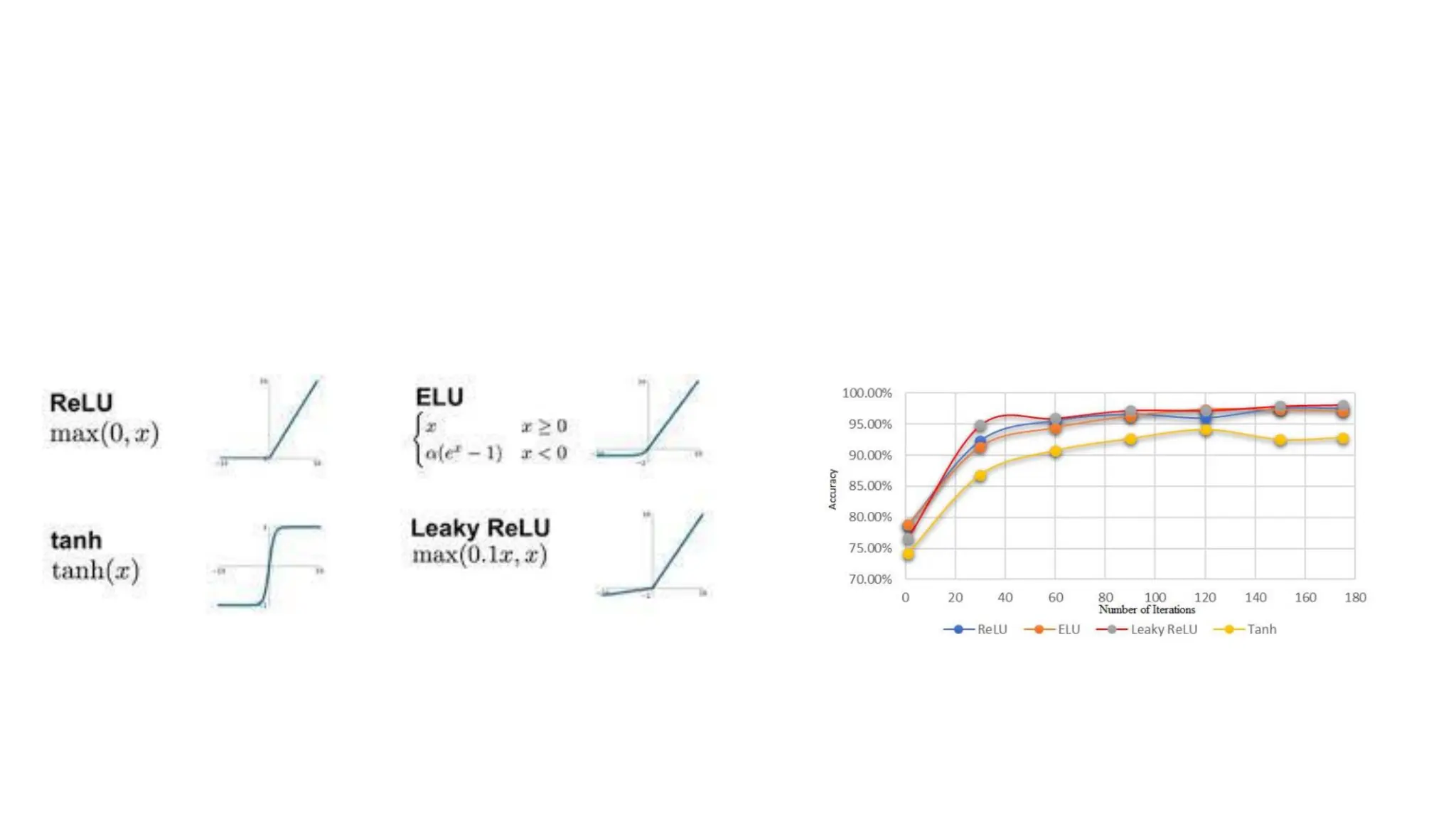
    ReLU (Rectified LinearUnit) • It gives an output x if x is positive and 0 otherwise. • It is derivable, but It is non-differentiable at 0. • It suffers from the dying ReLU problem (when output is negative). • ReLU is always going to discard the negative values
  • 18.
    Leaky ReLU • αis a small constant (normally 0.01). • Advantages: • it enjoys similar advantages to ReLU. • If the input is negative, the gradient will be α. As a result, there will be learning for these units as well. • Disadvantage: • the value of α is always constant and is a hyperparameter (parametric ReLU).
  • 19.
    ELU (Exponential LinearUnit) • Advantages: • ELU becomes smooth slowly until its output equal to -α whereas RELU sharply smoothes. This smoothness plays a beneficial role in optimization and generalization. • Unlike ReLU, It is derivable at 0. • Avoids dead ReLU problem by introducing log curve for negative values of input. • Disadvantages: • It is computationally expensive due to the presence of the exponential term. • α is a hyperparameter
  • 21.
    Regularization • it isoften convenient to explicitly introduce a regularization term (𝑅) which maps 𝑓 to a real number 𝑟 ∈ R. This term is usually used for penalizing the complexity of the model in the optimization • In practice, the family of functions chosen for the optimization can be parameterized by a parameter vector Θ, which allows the minimization to be defined as an exploration in the parameter space:
  • 22.
    • Regularization isa technique used in machine learning to prevent overfitting. • Overfitting happens when a model learns the training data too well, including the noise and outliers, which causes it to perform poorly on new data. • In simple terms, regularization adds a penalty to the model for being too complex, encouraging it to stay simpler and more general. This way, it’s less likely to make extreme predictions based on the noise in the data. • Regularization techniques help prevent overfitting by imposing constraints on the model’s parameters
  • 23.
    • This techniquehelps in several ways: • Complexity Control: Regularization reduces model complexity preventing overfitting and enhancing generalization to new data. • Balancing Bias and Variance: Regularization helps manage the trade-off between model bias (underfitting) and variance (overfitting) leading to better performance. • Feature Selection: Methods like L1 regularization (Lasso) encourage sparse solutions automatically selecting important features while excluding irrelevant ones. • Handling Multicollinearity: Regularization stabilizes models by reducing sensitivity to small changes when features are highly correlated. • Generalization: Regularized models focus on underlying patterns in the data ensuring better generalization rather than memorization. • In simple terms, regularization works like a guide that keeps the model from getting distracted by small, irrelevant details in the training data. By making the model simpler, regularization improves its ability to perform well on new, unseen data, rather than just memorizing the training data.
  • 24.
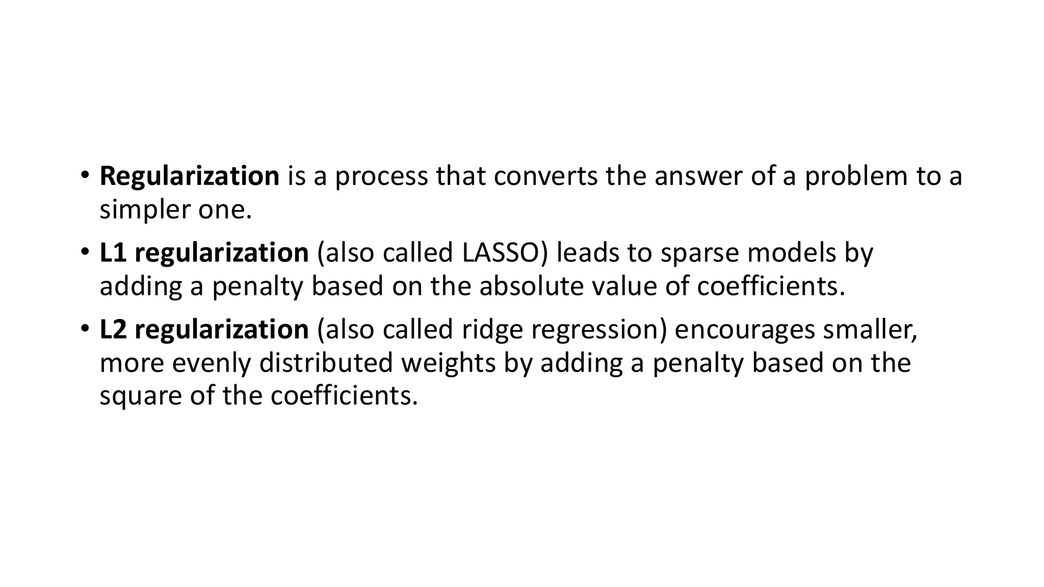
    • Regularization isa process that converts the answer of a problem to a simpler one. • L1 regularization (also called LASSO) leads to sparse models by adding a penalty based on the absolute value of coefficients. • L2 regularization (also called ridge regression) encourages smaller, more evenly distributed weights by adding a penalty based on the square of the coefficients.
  • 25.
    Regularization for regression •1. Lasso Regularization – (L1 Regularization) • 2. Ridge Regularization – (L2 Regularization) • 3. Elastic Net Regularization – (L1 and L2 Regularization)
  • 26.
    LASSO • A regressionmodel which uses the L1 Regularization technique is called LASSO(Least Absolute Shrinkage and Selection Operator) regression. • Lasso Regression adds the “absolute value of magnitude” of the coefficient as a penalty term to the loss function(L). • Lasso regression also helps us achieve feature selection by penalizing the weights to approximately equal to zero if that feature does not serve any purpose in the model.
  • 27.
    Ridge • A regressionmodel that uses the L2 regularization technique is called Ridge regression. • Ridge regression adds the “squared magnitude” of the coefficient as a penalty term to the loss function(L).
  • 28.
    Elastic Net • ElasticNet Regression is a combination of both L1 as well as L2 regularization. • That implies that we add the absolute norm of the weights as well as the squared measure of the weights. • With the help of an extra hyperparameter that controls the ratio of the L1 and L2 regularization. •α = 1 corresponds to Lasso (L1) regularization •α = 0 corresponds to Ridge (L2) regularization •Values between 0 and 1 provide a balance of both L1 and L2 regularization
  • 29.
    Regularization for NeuralNetworks • Weight decay is a regularization technique that operates by subtracting a fraction of the previous weights when updating the weights during training, effectively making the weights smaller over time. • Unlike L2 regularization which adds a penalty terms to the loss function, weight decay directly influences the weight update step itself. • This subtraction of a portion of the existing weights ensures that during each iteration of training, the model’s parameters are nudged towards smaller values. • where λ is a value determining the strength of the penalty (encouraging smaller weights).
  • 30.
    Weight decay • Inthe context of SGD, weight decay and L2 regularization are equivalent. This equivalence arises from the fact that the gradient of the L2 regularization term leads to the same parameter update as the one applied in weight decay. Therefore, in vanilla SGD, using either weight decay or L2 regularization will achieve the same result in terms of weight updates. And this is exactly the reason why the two terms have been used synonymously. • The paper by Loshchilov and Hutter (Link to PDF) conducted several experiments showing that weight decay performs significantly better than L2 regularization when used with Adam and other adaptive optimizers. Consequently, researchers and practitioners now commonly use a modified version of Adam called AdamW, which incorporates weight decay directly into the optimizer
  • 31.
    DropOut • In thecontext of neural networks, the Dropout technique repeatedly ignores random subsets of neurons during training, which simulates the training of multiple neural network architectures at once to improve generalization
  • 32.
  • 33.
    Best Practices forFine-Tuning • Gradual Unfreezing: Rather than fine-tuning all layers at once, gradually unfreeze the pre-trained layers starting from the top. This can lead to better performance and less risk of catastrophic forgetting. • Learning Rate Scheduling: Implement learning rate scheduling to decrease the learning rate gradually as training progresses. This approach can help in achieving better fine-tuning results. • Data Augmentation: For tasks such as image classification, data augmentation techniques (e.g., cropping, rotation) can effectively increase the size of your training dataset, helping the model generalize better. • Regularization Techniques: Utilize regularization techniques like dropout and weight decay to prevent overfitting, especially when your task-specific dataset is relatively small.
  • 34.
    PEFT • Parameter-efficient fine-tuning(PEFT) is a language model fine-tuning technique specifically designed to update only a small portion of the model’s parameters instead of all of the parameters. It alleviates the computational problem and catastrophic forget problem that full fine-tuning has. • The most famous technique within PEFT is LoRA (Low-Rank Adaptation). • It’s a method for adapting a pre-trained model by injecting low-rank matrices into the model’s layer to modify certain parts’ behavior while keeping the original parameters frozen. • This technique is valuable and has been proven to alter the pre-trained model. •
  • 35.
    Instruction Tuning • Instructiontuning is a fine-tuning technique for the pre-trained model to follow natural language directions for various tasks. • instruction tuning usually does not focus on specific tasks; instead, it uses a dataset that includes diverse tasks that were formatted as instructions with the expected output.