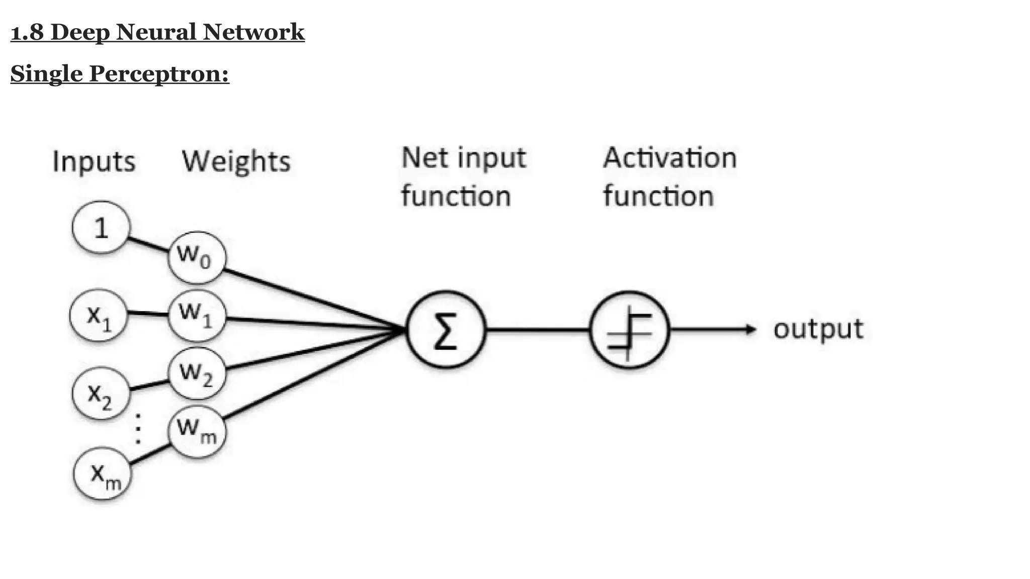
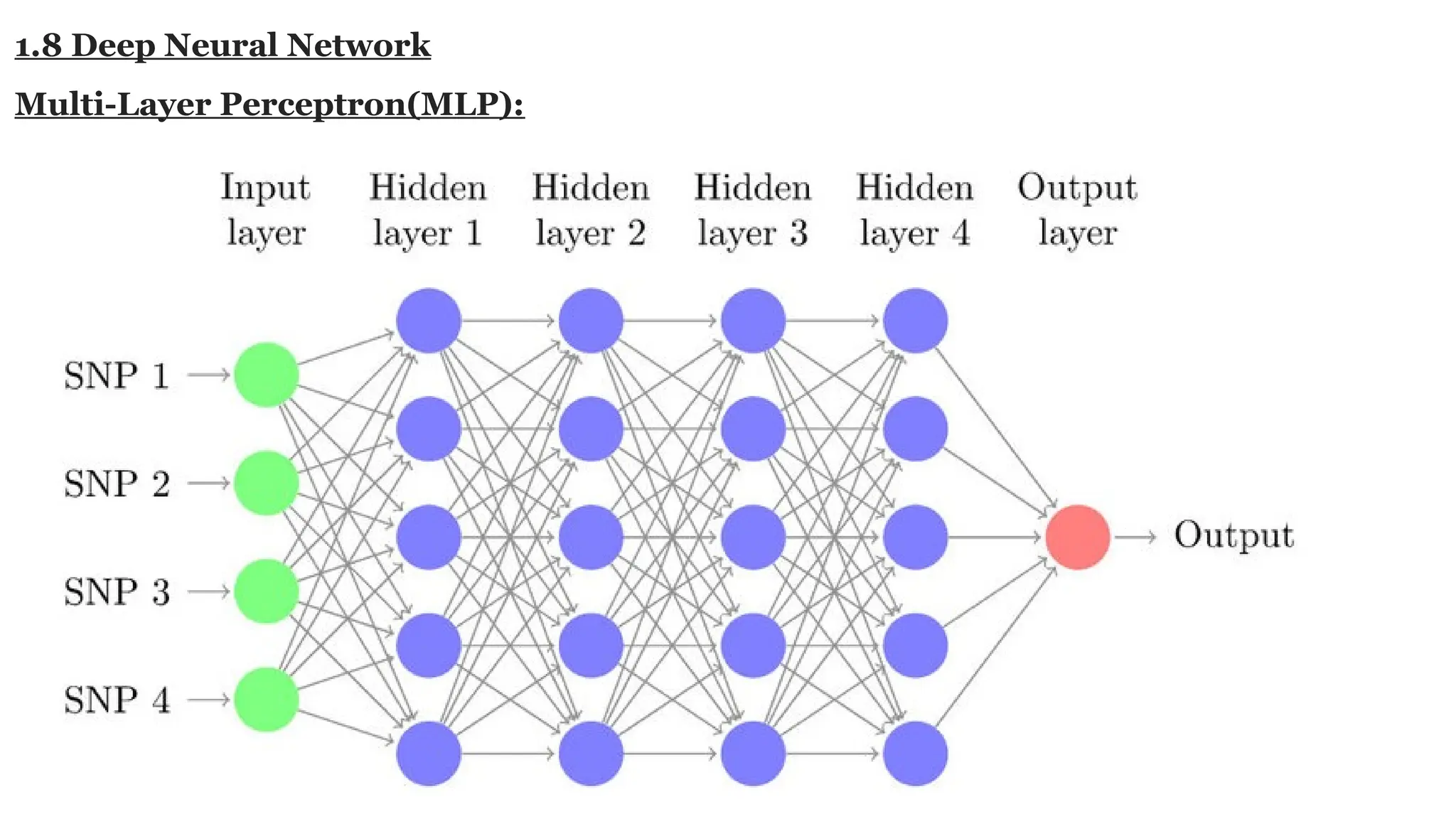
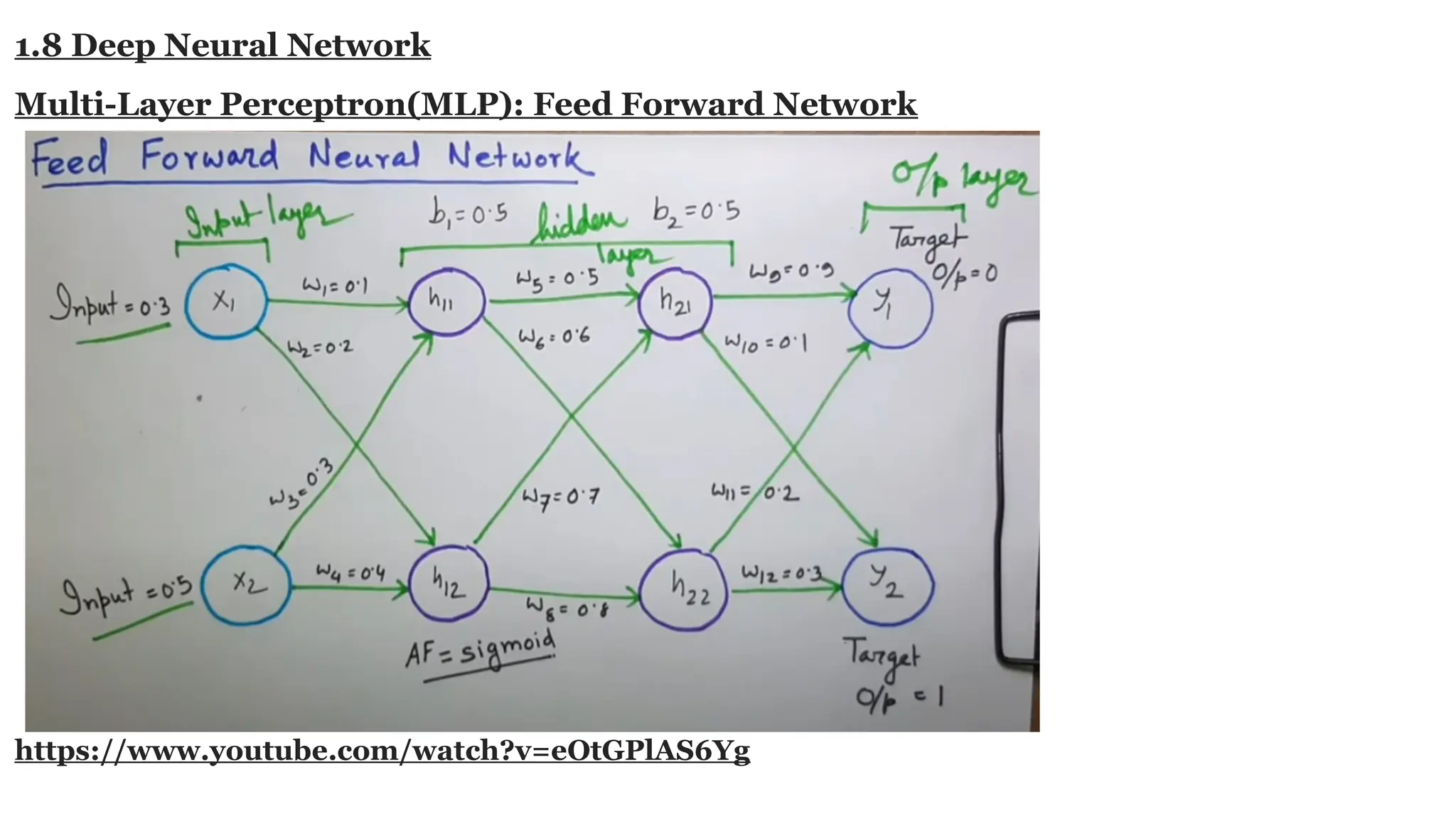
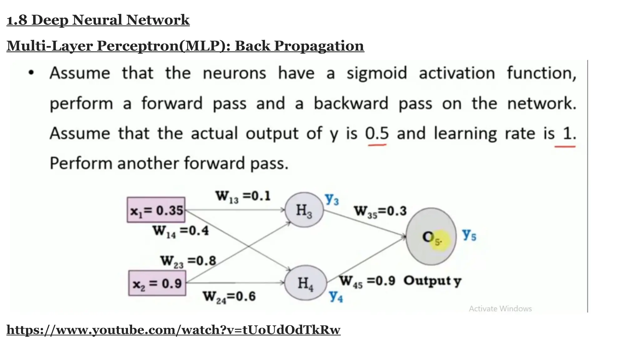
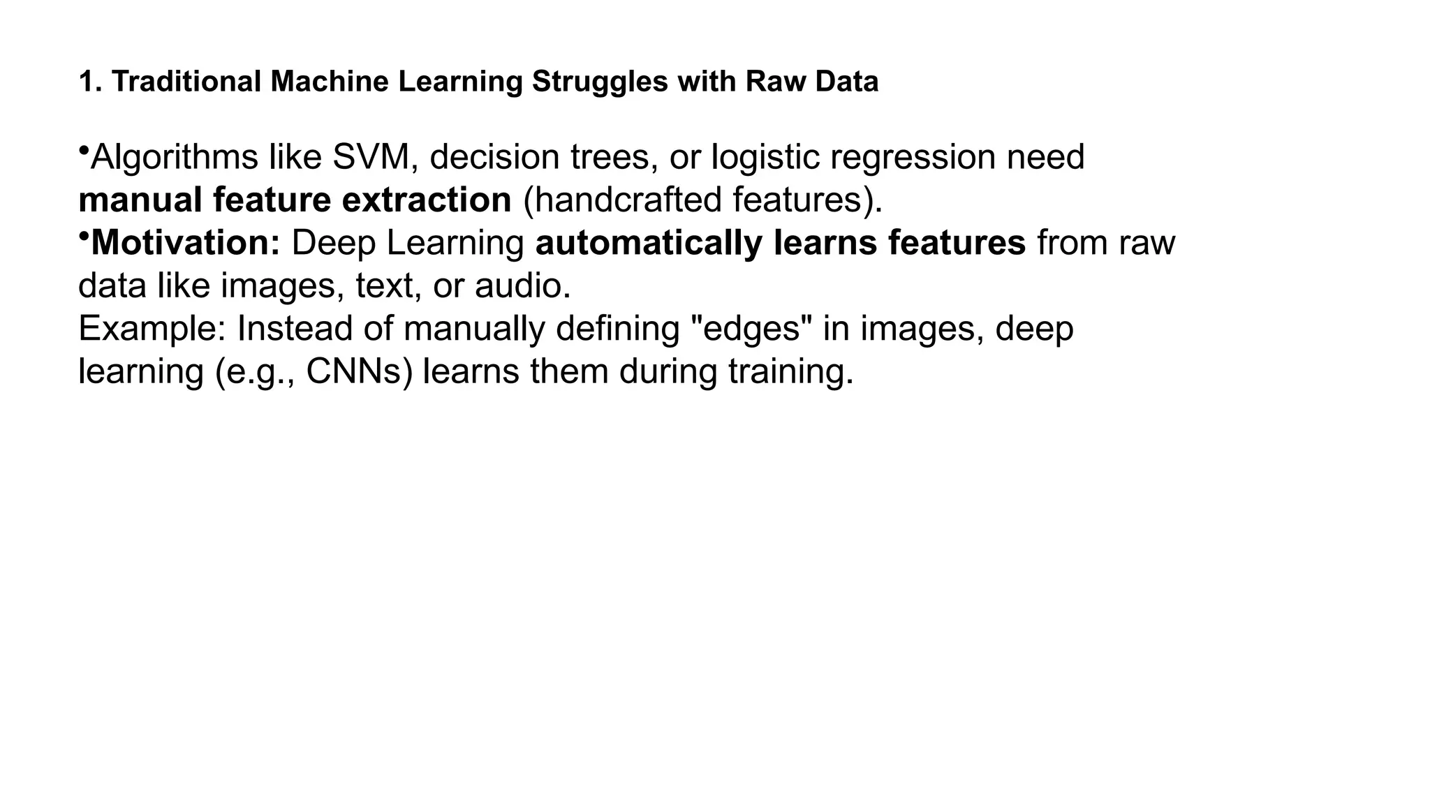
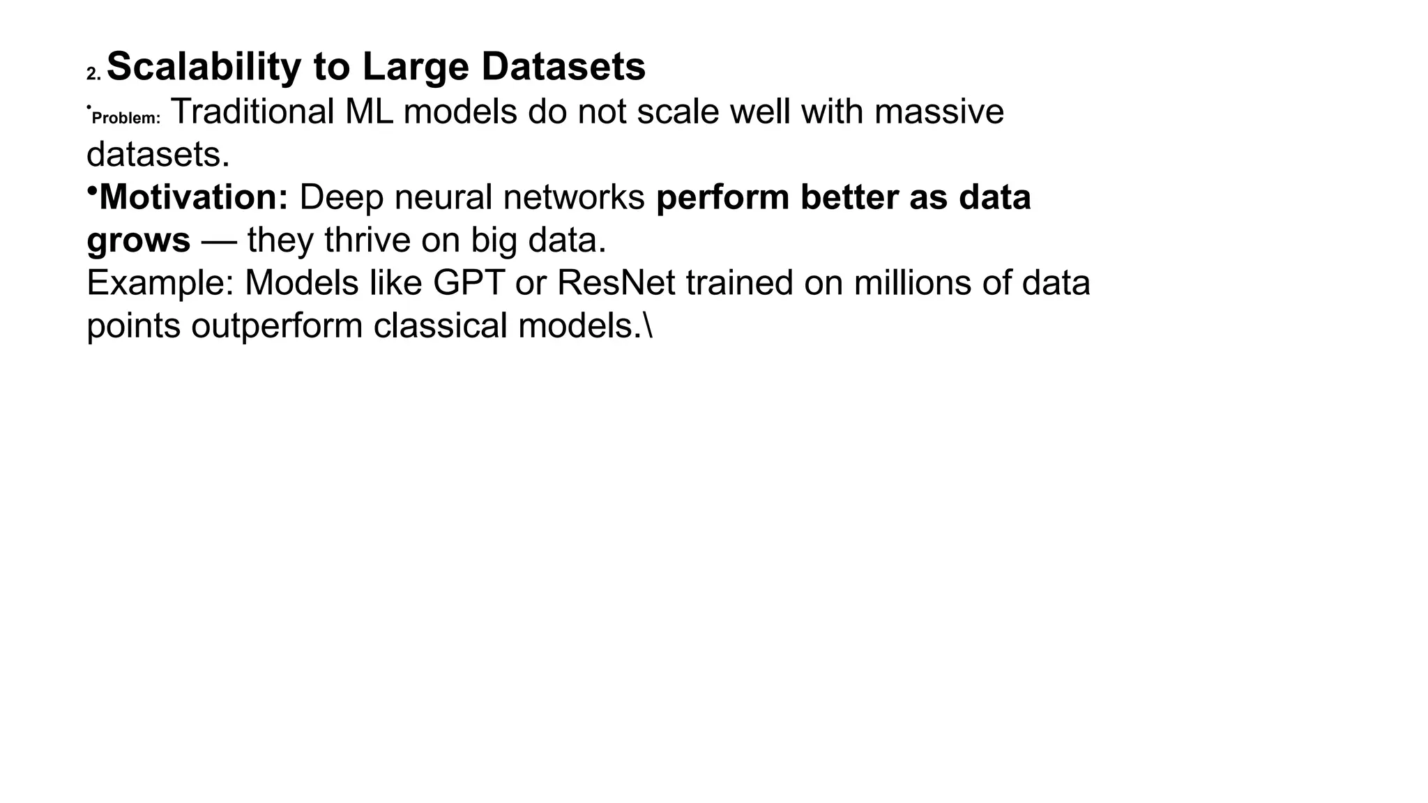
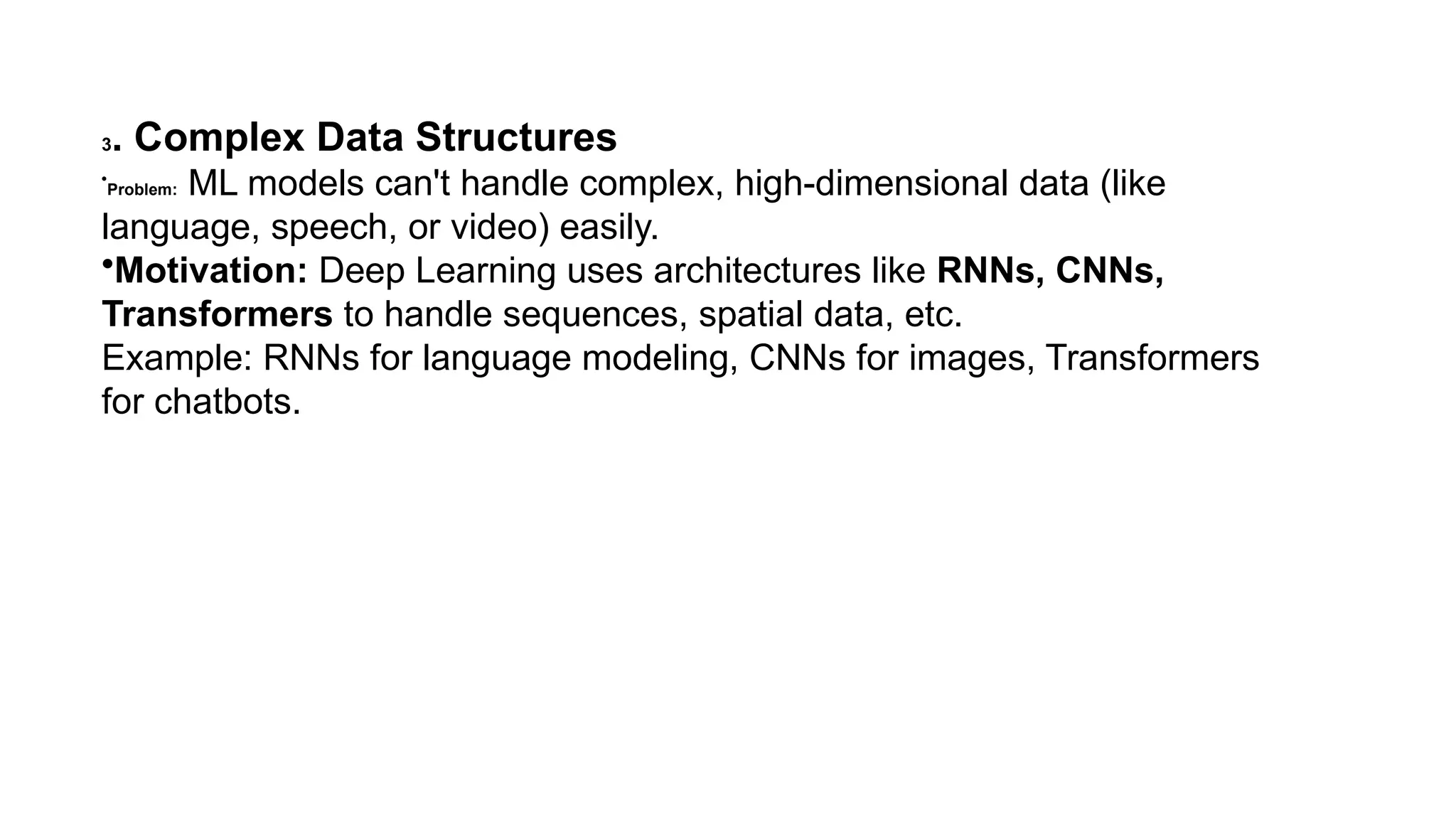
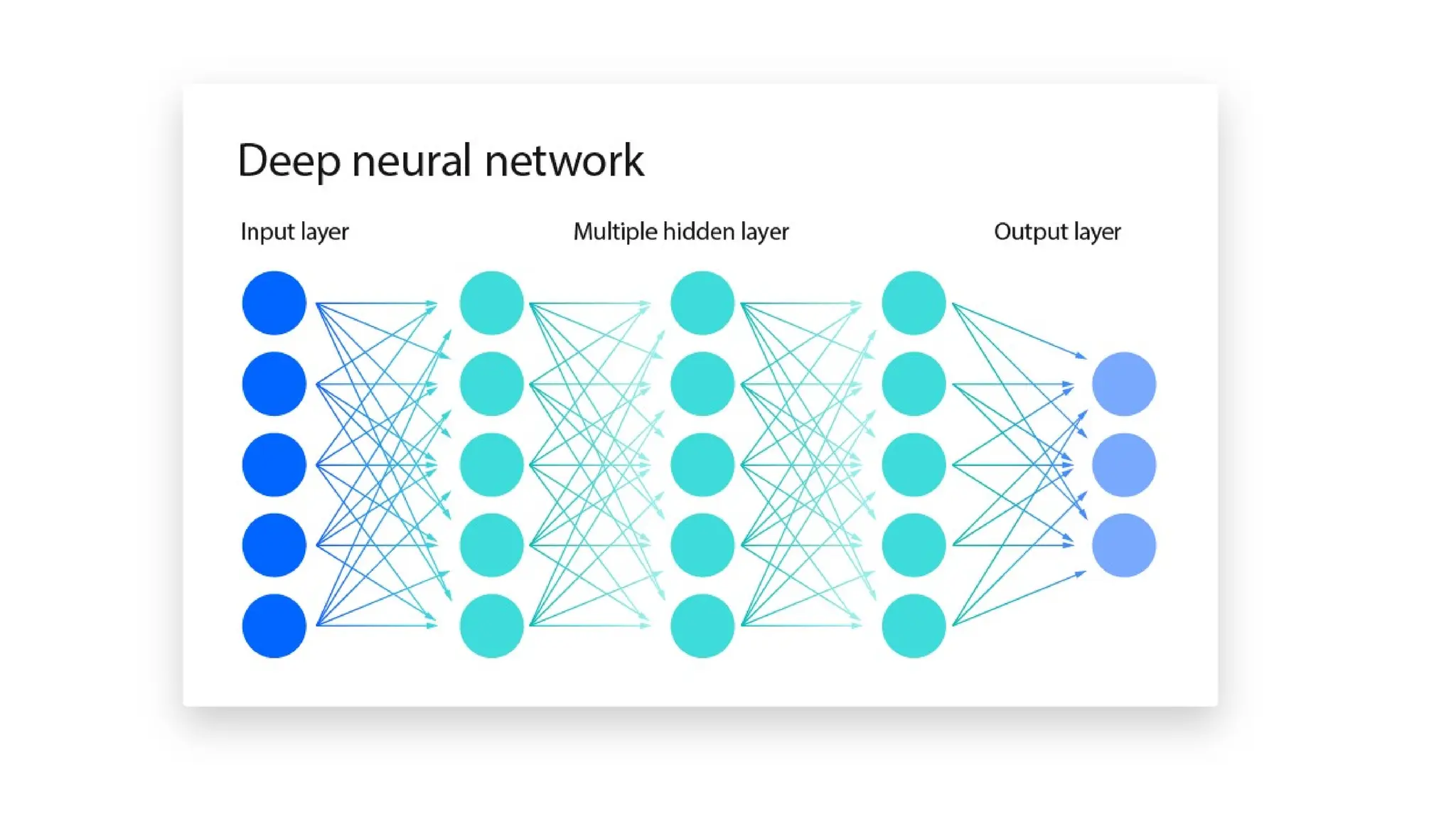
machine learning that uses artificial neural networks with multiple hidden layers to learn from vast amounts of data

UNIT I - DEEP NETWORKS BASICS 1.1 Linear Algebra: Scalars, Vectors, Matrices, tensors Linear Algebra for Deep Learning: The Math behind every deep learning program. Deep Learning is a subdomain of machine learning, concerned with the algorithm which imitates the function and structure of the brain called the artificial neural network. Linear algebra is a form of continuous rather than discrete mathematics, many computer scientists have little experience with it. A good understanding of linear algebra is essential for understanding and working with many machine learning algorithms, especially deep learning algorithms. A linear equation is an equation in which the highest power of the variable is always 1. It is also known as a one-degree equation. The standard form of a linear equation in one variable is of the form Ax + B = 0. Here, x is a variable, A is a coefficient and B is constant.

When confined to smaller levels, everything is math behind deep learning. So it is essential to understand basic linear algebra before getting started with deep learning and programming it. Scalars Scalars are single numbers and are an example of a 0th-order tensor. The notation x states that x is ∈ ℝ a scalar belonging to a set of real-values numbers, ℝ

Few built-in scalar types are int, float, complex, bytes, Unicode in Python. In In NumPy a python library, there are 24 new fundamental data types to describe different types of scalars. Vectors Vectors are ordered arrays of single numbers and are an example of 1st-order tensor. fragments of objects known as vector spaces. Matrices Matrices are rectangular arrays consisting of numbers and are an example of 2nd-order tensors. If m and n are positive integers, that is m, n then the m×n matrix contains m*n numbers, with m rows and n ∈ ℕ columns. The full m×n matrix can be written as:

Tensors The more general entity of a tensor encapsulates the scalar, vector and the matrix. It is sometimes necessary — both in the physical sciences and machine learning — to make use of tensors with order that exceeds two. We use Python libraries like tensorflow or PyTorch in order to declare tensors, rather than nesting matrices.

1.2 Probability Distributions Probability Distribution is basically the set of all possible outcomes of any random experiment or event. Different Types of Probability Distributions: ● Discrete Probability Distributions for discrete variables ● Cumulative Probability Distribution for continuous variables

Continuous Distributions These represent outcomes that can take any real value within a range. 1.Uniform •All values between a and b are equally likely. •Example: Picking a random number between 0 and 1. 2.Exponential •Models the time between events in a Poisson process. Example: Time until the next earthquake. 3. Normal (Gaussian) Bell-shaped curve; most values are near the average (mean). Example: Heights of people, test scores.

Discrete Distributions These represent outcomes that take specific, countable values. Binomial Number of successes in a fixed number of trials. Example: Tossing a coin 10 times and counting heads. Geometric Counts how many trials until the first success. Example: How many times you roll a die until you get a 6. Hypergeometric Like binomial, but without replacement. Example: Drawing cards from a deck without putting them back.

1.2 Probability Distributions Types of distributions: Common distributions used in deep learning include: ● Normal distribution (bell-shaped curve): For continuous outputs, like predicting house prices. ● Bernoulli distribution (binary outcomes): For classification tasks, like image recognition (cat vs. dog). ● Categorical distribution (multiple categories): When there are more than two classes, like recognizing different types of flowers.

1.2 Probability Distributions Binary outcomes formula Categorical Distribution Formula

1.3 Gradient-based Optimization

Types of Gradient Descent 1. Batch Gradient Descent: Batch gradient descent (BGD) is used to find the error for each point in the training set and update the model after evaluating all training examples. This procedure is known as the training epoch. In simple words, it is a greedy approach where we have to sum over all examples for each update. 2. Stochastic gradient descent Stochastic gradient descent (SGD) is a type of gradient descent that runs one training example per iteration. Or in other words, it processes a training epoch for each example within a dataset and updates each training example's parameters one at a time. 3. MiniBatch Gradient Descent: Mini Batch gradient descent is the combination of both batch gradient descent and stochastic gradient descent. It divides the training datasets into small batch sizes then performs the updates on those batches separately Challenges with the Gradient Descent 1. Local Minima and Saddle Point, 2. Vanishing and Exploding Gradient

1.4 Machine Learning Basics Machine learning (ML) is a branch of artificial intelligence (AI) and computer science that focuses on the using data and algorithms to enable AI to imitate the way that humans learn, gradually improving its accuracy.

1.4 Machine Learning Basics (Capacity Overfitting and Underfitting) 1.4.1 Overfitting

ML | Underfitting and Overfitting Machine learning models aim to perform well on both training data and new, unseen data and is considered "good" if: It learns patterns effectively from the training data. It generalizes well to new, unseen data. It avoids memorizing the training data (overfitting) or failing to capture relevant patterns (underfitting).

Contd.. To evaluate how well a model learns and generalizes, we monitor its performance on both the training data and a separate validation or test dataset which is often measured by itsaccuracy or prediction errors. However, achieving this balance can be challenging. Two common issues that affect a model's performance and generalization ability are overfitting and underfitting. These problems are major contributors to poor performance in machine learning models. Let's us understand what they are and how they contribute to ML models.

Bias and Variance in Machine Learning Bias and variance are two key sources of error in machine learning models that directly impact their performance and generalization ability. Bias: is the error that happens when a machine learning model is too simple and doesn't learn enough details from the data. It's like assuming all birds can only be small and fly, so the model fails to recognize big birds like ostriches or penguins that can't fly and get biased with predictions.

These assumptions make the model easier to train but may prevent it from capturing the underlying complexities of the data. High bias typically leads to underfitting, where the model performs poorly on both training and testing data because it fails to learn enough from the data. Example: A linear regression model applied to a dataset with a non-linear relationship.

Variance: Error that happens when a machine learning model learns too much from the data, including random noise. A high-variance model learns not only the patterns but also the noise in the training data, which leads to poor generalization on unseen data. High variance typically leads to overfitting, where the model performs well on training data but poorly on testing data.

Overfitting and Underfitting: The Core Issues 1. Overfitting in Machine Learning Overfitting happens when a model learns too much from the training data, including details that don’t matter (like noise or outliers). For example, imagine fitting a very complicated curve to a set of points. The curve will go through every point, but it won’t represent the actual pattern. As a result, the model works great on training data but fails when tested on new data. Overfitting models are like students who memorize answers instead of understanding the topic. They do well in practice tests (training) but struggle in real exams (testing).

2. Underfitting in Machine Learning Underfitting is the opposite of overfitting. It happens when a model is too simple to capture what’s going on in the data. For example, imagine drawing a straight line to fit points that actually follow a curve. The line misses most of the pattern. In this case, the model doesn’t work well on either the training or testing data. Underfitting models are like students who don’t study enough. They don’t do well in practice tests or real exams.Note: The underfitting model has High bias and low variance.

Reasons for Overfitting: High variance and low bias. The model is too complex. The size of the training data. Reasons for Underfitting: The model is too simple, So it may be not capable to represent the complexities in the data. The input features which is used to train the model is not the adequate representations of underlying factors influencing the target variable. The size of the training dataset used is not enough. Excessive regularization are used to prevent the overfitting, which constraint the model to capture the data well. Features are not scaled.

Techniques to Reduce Underfitting Increase model complexity. Increase the number of features, performing feature engineering. Remove noise from the data. Increase the number of epochs or increase the duration of training to get better results. Techniques to Reduce Overfitting Improving the quality of training data reduces overfitting by focusing on meaningful patterns, mitigate the risk of fitting the noise or irrelevant features. Increase the training data can improve the model's ability to generalize to unseen data and reduce the likelihood of overfitting. Reduce model complexity. Early stopping during the training phase (have an eye over the loss over the training period as soon as loss begins to increase stop training). Ridge Regularization and Lasso Regularization. Use dropout for neural networks to tackle overfitting

1.4 Machine Learning Basics (Capacity Overfitting and Underfitting High Variance Low Variance, Low Bias High Bias

1.4 Machine Learning Basics (Capacity Overfitting and Underfitting)

Hyperparameters Hyperparameters are parameters whose values control the learning process and determine the values of model parameters that a learning algorithm ends up learning. The prefix ‘hyper_’ suggests that they are ‘top-level’ parameters that control the learning process and the model parameters that result from it. As a machine learning engineer designing a model, you choose and set hyperparameter values that your learning algorithm will use before the training of the model even begins. In this light, hyperparameters are said to be external to the model because the model cannot change its values during learning/training.

Hyperparameters are used by the learning algorithm when it is learning but they are not part of the resulting model. At the end of the learning process, we have the trained model parameters which effectively is what we refer to as the model. The hyperparameters that were used during training are not part of this model. We cannot for instance know what hyperparameter values were used to train a model from the model itself, we only know the model parameters that were learned. Basically, anything in machine learning and deep learning that you decide their values or choose their configuration before training begins and whose values or configuration will remain the same when training ends is a hyperparameter.

Here are some common examples Train-test split ratio Learning rate in optimization algorithms (e.g. gradient descent) Choice of optimization algorithm (e.g., gradient descent, stochastic gradient descent, or Adam optimizer) Choice of activation function in a neural network (nn) layer (e.g. Sigmoid, ReLU, Tanh) The choice of cost or loss function the model will use Number of hidden layers in a nn

Number of activation units in each layer The drop-out rate in nn (dropout probability) Number of iterations (epochs) in training a nn Number of clusters in a clustering task Kernel or filter size in convolutional layers Pooling size Batch size

1.8 Deep Neural Network Single Perceptron:

1.8 Deep Neural Network Multi-Layer Perceptron(MLP):

1.8 Deep Neural Network Multi-Layer Perceptron(MLP): Feed Forward Network https://www.youtube.com/watch?v=eOtGPlAS6Yg

1.8 Deep Neural Network Multi-Layer Perceptron(MLP): Back Propagation https://www.youtube.com/watch?v=tUoUdOdTkRw

Gradient descent is the backbone of the learning process for various algorithms, including linear regression, logistic regression, support vector machines, and neural networks which serves as a fundamental optimization technique to minimize the cost function of a model by iteratively adjusting the model parameters to reduce the difference between predicted and actual values, improving the model's performance.

Introduction to Gradient Descent Gradient Descent is an algorithm used to find the best solution to a problem by making small adjustments in the right direction. It’s like trying to find the lowest point in a hilly area by walking down the slope, step by step, until you reach the bottom.

Imagine you're at the top of a hill and your goal is to find the lowest point in the valley. You can't see the entire valley from the top, but you can feel the slope under your feet. Start at the Top: You begin at the top of the hill (this is like starting with random guesses for the model's parameters). Feel the Slope: You look around to find out which direction the ground is sloping down. This is like calculating the gradient, which tells you the steepest way downhill. Take a Step Down: Move in the direction where the slope is steepest (this is adjusting the model's parameters). The bigger the slope, the bigger the step you take. Repeat: You keep repeating the process — feeling the slope and moving downhill — until you reach the bottom of the valley (this is when the model has learned and minimized the error).

ML - Stochastic Gradient Descent (SGD) ● Stochastic Gradient Descent (SGD) is an optimization algorithm in machine learning, particularly when dealing with large datasets. It is a variant of the traditional gradient descent algorithm but offers several advantages in terms of efficiency and scalability, making it the go-to method for many deep-learning tasks.

Need for Stochastic Gradient Descent ● For large datasets, computing the gradient using all data points can be slow and memory- intensive. This is where SGD comes into play. Instead of using the full dataset to compute the gradient at each step, SGD uses only one random data point (or a small batch of data points) at each iteration. This makes the computation much faster.

Working of Stochastic Gradient Descent ● In Stochastic Gradient Descent, the gradient is calculated for each training example (or a small subset of training examples) rather than the entire dataset. ● The update rule becomes:

Implementing Stochastic Gradient Descent from Scratch 1. Generating the Data In this step, we generate synthetic data for the linear regression problem. The data consists of feature X and the target y, where the relationship is linear, i.e., y = 4 + 3 * X + noise. •X is a random array of 100 samples between 0 and 2. •y is the target, calculated using a linear equation with a little random noise to make it more realistic.

1. Traditional Machine Learning Struggles with Raw Data •Algorithms like SVM, decision trees, or logistic regression need manual feature extraction (handcrafted features). •Motivation: Deep Learning automatically learns features from raw data like images, text, or audio. Example: Instead of manually defining "edges" in images, deep learning (e.g., CNNs) learns them during training.

2. Scalability to Large Datasets • Problem: Traditional ML models do not scale well with massive datasets. •Motivation: Deep neural networks perform better as data grows — they thrive on big data. Example: Models like GPT or ResNet trained on millions of data points outperform classical models.

3. Complex Data Structures • Problem: ML models can't handle complex, high-dimensional data (like language, speech, or video) easily. •Motivation: Deep Learning uses architectures like RNNs, CNNs, Transformers to handle sequences, spatial data, etc. Example: RNNs for language modeling, CNNs for images, Transformers for chatbots.

Poor Generalization on Unseen Data Problem: Traditional models often overfit or underfit. Motivation: Deep learning, with proper regularization and architectures, generalizes better when trained with enough data.

Multimodal Data Integration • Problem: Hard to combine different types of data (text + image + audio). •Motivation: Deep learning can fuse multiple data types effectively using joint representations. Example: Self-driving cars process video, LIDAR, audio, etc., simultaneously.

End-to-End Learning Desire Problem: ML pipelines had many disconnected stages (feature extraction → model → post-processing). Motivation: Deep learning allows end-to-end training, reducing complexity and error propagation.

Feedback Neural Networks: Structure, Training, and Applications Neural networks, a cornerstone of deep learning, are designed to simulate the human brain's behavior in processing data and making decisions. Among the various types of neural networks, feedback neural networks (also known as recurrent neural networks or RNNs) play a crucial role in handling sequential data and temporal dynamics. This article delves into the technical aspects of feedback neural networks, their structure, training methods, and applications.

What is a Neural Network? A neural network is a computational model inspired by the human brain's network of neurons. It consists of layers of interconnected nodes (neurons) that process input data to produce an output. Neural networks are used in various applications, from image and speech recognition to natural language processing and autonomous systems.

Types of Neural Networks Neural networks can be broadly classified into two categories: Feedforward Neural Networks (FNNs): These networks have a unidirectional flow of information from input to output, with no cycles or loops. They are typically used for tasks like image classification and regression. Feedback Neural Networks (RNNs): These networks have connections that loop back, allowing information to be fed back into the network. This structure enables them to handle sequential data and temporal dependencies, making them suitable for tasks like time series prediction and language modeling.

Structure of Feedback Neural Networks Feedback neural networks, or RNNs, are characterized by their ability to maintain a state that captures information about previous inputs. This is achieved through recurrent connections that loop back from the output to the input of the same layer or previous layers. The key components of an RNN include: Input Layer: Receives the input data. Hidden Layers: Contain neurons with recurrent connections that maintain a state over time. Output Layer: Produces the final output based on the processed information.

Mechanisms of Feedback in Neural Networks There are several mechanisms by which feedback is implemented in neural networks. These include: Backpropagation: Backpropagation is a method of feedback that involves the computation of the error gradient at each layer of the network. The error gradient is then used to update the network's parameters. Backpropagation is widely used in deep neural networks due to its efficiency and accuracy. Recurrent Connections: Recurrent connections involve the feedback of information from a later stage of the network to an earlier stage. This type of feedback is used in recurrent neural networks (RNNs), which are designed to handle sequential data. Lateral Connections: Lateral connections involve the feedback of information between neurons in the same layer. This type of feedback is used in applications such as image processing, where the goal is to capture spatial relationships between pixels.

Learning in Feedback Networks: Embracing Backpropagation Through Time (BPTT) Training feedback networks presents a unique challenge compared to feedforward networks. The traditional backpropagation algorithm cannot be directly applied due to the presence of loops. Here, backpropagation through time (BPTT) comes into play. BPTT unfolds the recurrent network over time, essentially creating a temporary feed-forward architecture for each sequence element. The error signal is then propagated backward through this unfolded network, allowing the network to adjust its weights and learn from the feedback. However, BPTT can become computationally expensive for long sequences, necessitating the development of more efficient training algorithms. The steps involved in BPTT are:

Forward Pass: Compute the output of the network for each time step. Backward Pass: Compute the gradients of the loss function with respect to the weights by propagating the error backward through time. Weight Update: Adjust the weights using the computed gradients to minimize the loss. BPTT can be computationally expensive and suffer from issues like vanishing and exploding gradients, which can hinder the training of deep RNNs.

Applications of Feedback Neural Networks Feedback neural networks are well-suited for tasks involving sequential data and temporal dependencies. Some common applications include: Natural Language Processing (NLP): RNNs are used for tasks like language modeling, machine translation, and sentiment analysis, where the context and order of words are important. Time Series Prediction: RNNs can model temporal dependencies in time series data, making them useful for forecasting stock prices, weather, and other time-dependent phenomena. Speech Recognition: RNNs can process audio signals over time, enabling accurate transcription of spoken language. Handwriting Recognition: RNNs can recognize handwritten text by processing sequences of pen strokes.

Conclusion Feedback neural networks are a powerful tool for handling sequential data and temporal dependencies. Their ability to maintain a state over time makes them suitable for a wide range of applications, from natural language processing to time series prediction. Despite the challenges in training and scalability, ongoing research continues to advance the capabilities of feedback neural networks, paving the way for more sophisticated and efficient models in the future.

Imagine a cascade of filters, each specializing in detecting progressively more intricate features in your data. That's essentially how a deep network functions. 1.Input Layer: Receives the raw data, such as pixels from an image or words in a sentence. 2.Hidden Layers: Each hidden layer applies a set of mathematical operations, often nonlinear transformations, to the data it receives from the previous layer. 3.Feature Learning: The initial layers might identify basic features like edges or textures, while deeper layers learn to combine these basic features into more complex representations, such as objects or abstract concepts. 4.Output Layer: The final layer produces the network's prediction or classification based on the learned features. 5.Training and Adjustment: Deep networks learn by adjusting the "weights" and "biases" associated with the connections between neurons, based on the difference between the network's predictions and the desired output. This process, often involving backpropagation and optimization algorithms like gradient descent, iteratively refines the network's ability to accurately process information.

Key advantages of deep networks Automatic Feature Extraction: Unlike traditional machine learning techniques that require manual feature engineering, deep learning automatically discovers and learns relevant features directly from the data. Handling Complex & Unstructured Data: Deep networks excel at processing large volumes of complex and unstructured data, such as images, videos, text, and audio, according to IBM. High Accuracy & Performance: Deep learning has achieved state-of-the-art results in various tasks, including image recognition, speech recognition, and natural language processing. Learning Hierarchical Representations: The multiple layers allow deep networks to learn hierarchical representations of the data, which is crucial for understanding complex concepts and relationships.

Common types of deep networks Convolutional Neural Networks (CNNs): Primarily used for computer vision tasks, such as image recognition and object detection. Recurrent Neural Networks (RNNs): Designed for sequential data like time series and natural language processing tasks. Generative Adversarial Networks (GANs): Generate new data resembling the training data, used in applications like image generation and style transfer. Transformers: Revolutionized NLP with self-attention mechanisms, excelling at tasks like machine translation, text generation, and sentiment analysis.

Challenges and limitations Despite their remarkable capabilities, deep networks pose certain challenges: •Data Requirements: Deep learning models typically require vast amounts of high-quality data for effective training. •Computational Resources: Training deep networks is computationally intensive and demands significant processing power hardware like GPUs or TPUs. •Interpretability (Black Box Problem): Understanding how deep networks arrive at their predictions can be challenging, maki •Overfitting: Deep networks can be prone to overfitting, where they perform well on the training data but poorly on unseen

machine learning that uses artificial neural networks with multiple hidden layers to learn from vast amounts of data

machine learning that uses artificial neural networks with multiple hidden layers to learn from vast amounts of data

More Related Content

Similar to machine learning that uses artificial neural networks with multiple hidden layers to learn from vast amounts of data

More from jeevamahalakshmi

Recently uploaded

machine learning that uses artificial neural networks with multiple hidden layers to learn from vast amounts of data