Download to read offline

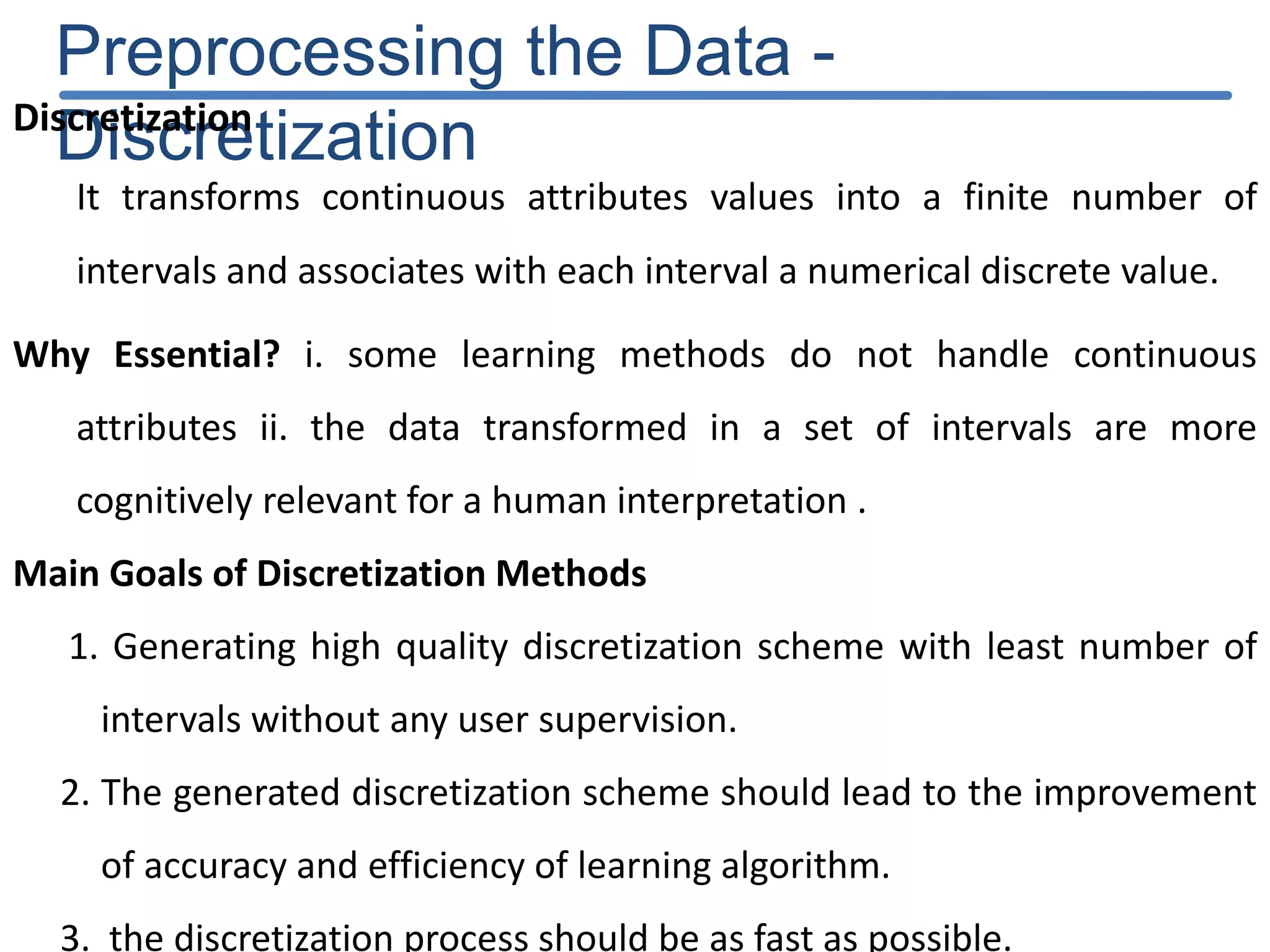
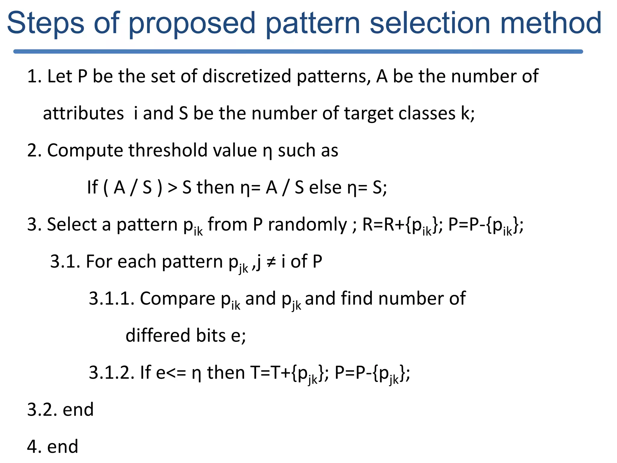
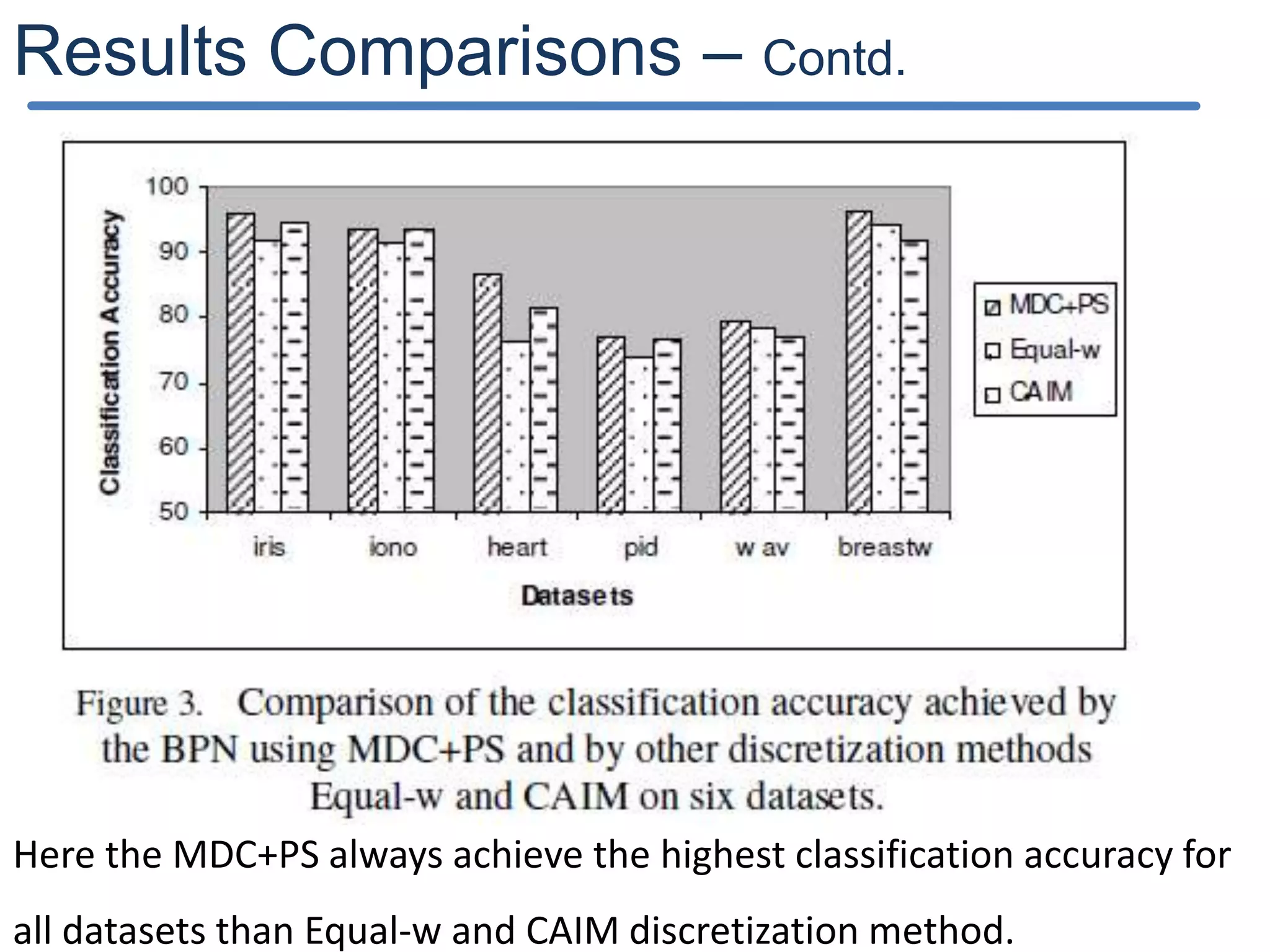
![Pattern Selection Method (PS) Pattern selection It is an active learning strategy to select the most informative patterns for training the network. It obtains a good training set to increase the performance of a neural network in terms of convergence speed and generalization. Proposed Pattern Selection (PS) method : A data which was discretized into many intervals by MDC is converted into binary code using the Thermometer coding scheme [27]. PS selects all distinct patterns based on pattern disparity for training the feedforward neural network.](https://image.slidesharecdn.com/presentationforviva-200509174241/75/Novel-algorithms-for-Knowledge-discovery-from-neural-networks-in-Classification-problems-11-2048.jpg)
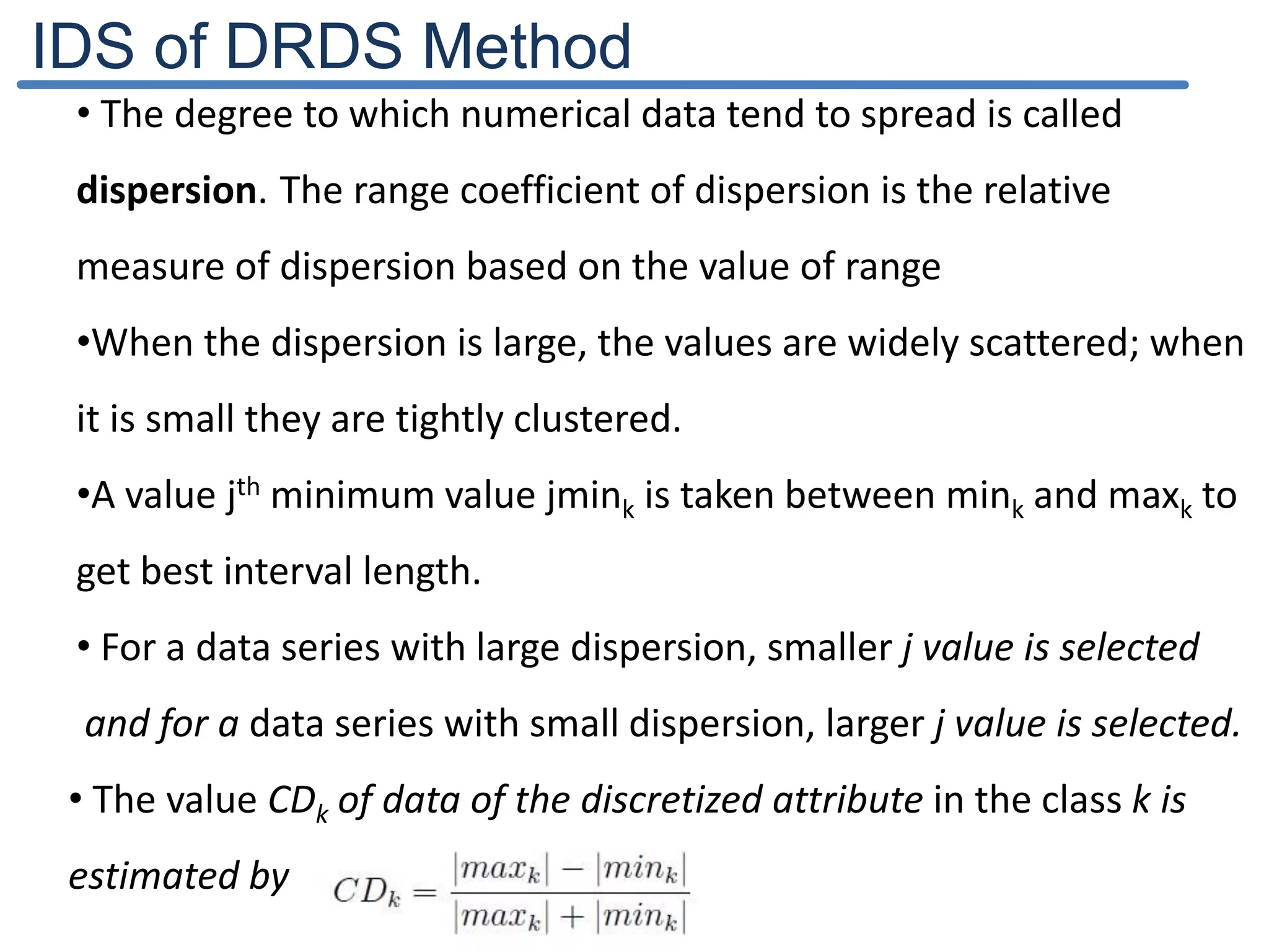
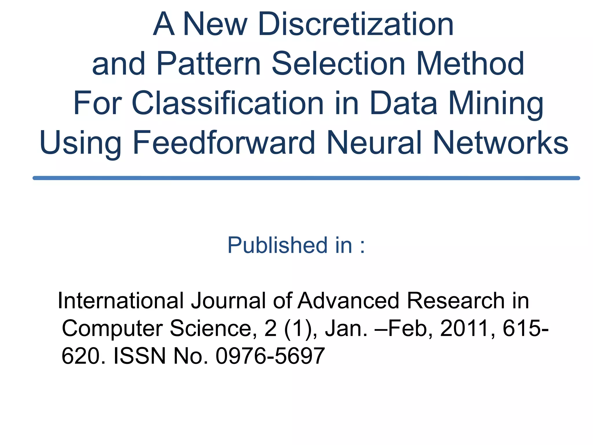
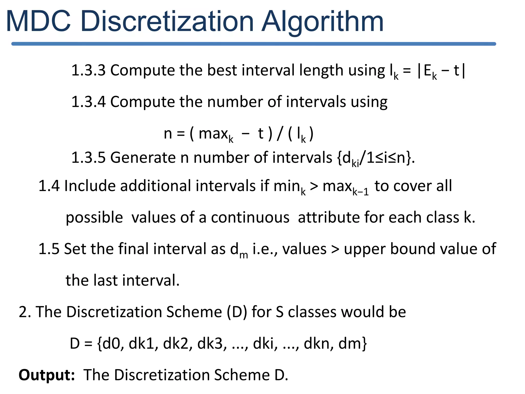
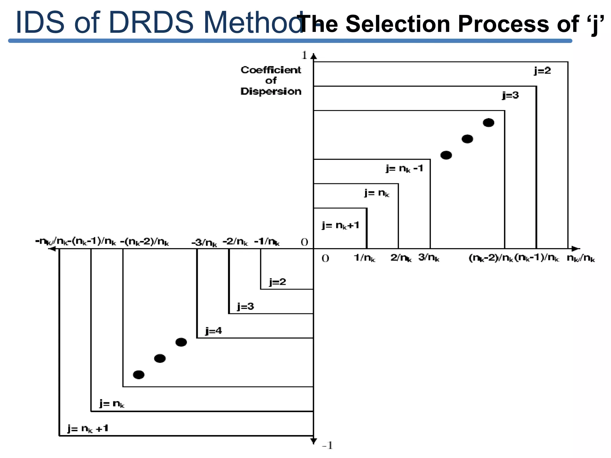
![IDS of DRDS Method The value of CDk is always in [-1; +1]. To decide the value j, the range [-1; +1] is divided into set of intervals based on the magnitude of number of distinct values in the discretizing attribute of the class k. The value j is selected based on the value of CDk lies in the above interval. The best interval length lk for a discretizing attribute of a class k can be obtained by, A distribution of data is said to be skewed if the given data is symmetrical but stretched more to one side than to the other. The selection of very small jmink value due to the right skewness leads the interval length lk as too small and the number of intervals n also as very high vice versa. This adjustment process of lk can be formulated as,](https://image.slidesharecdn.com/presentationforviva-200509174241/75/Novel-algorithms-for-Knowledge-discovery-from-neural-networks-in-Classification-problems-20-2048.jpg)
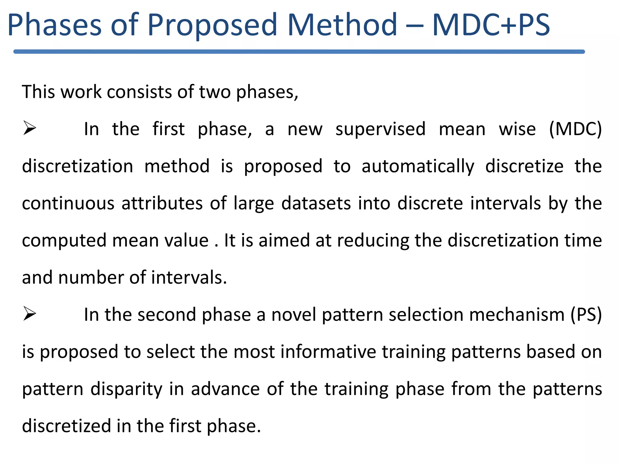
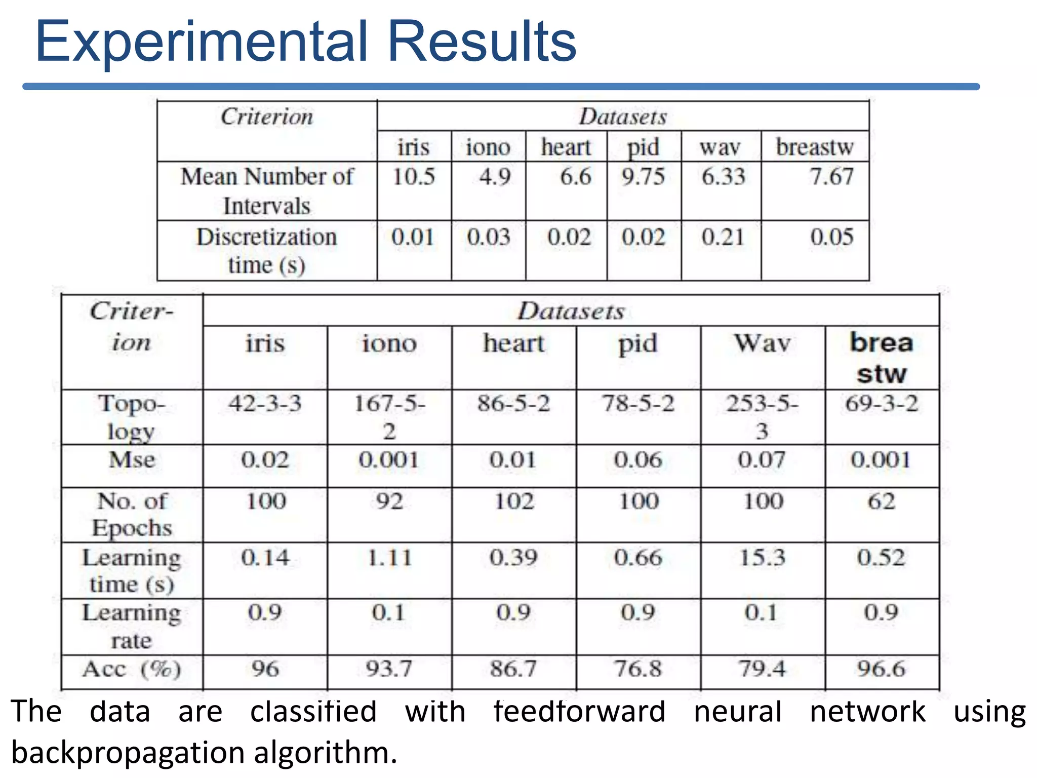
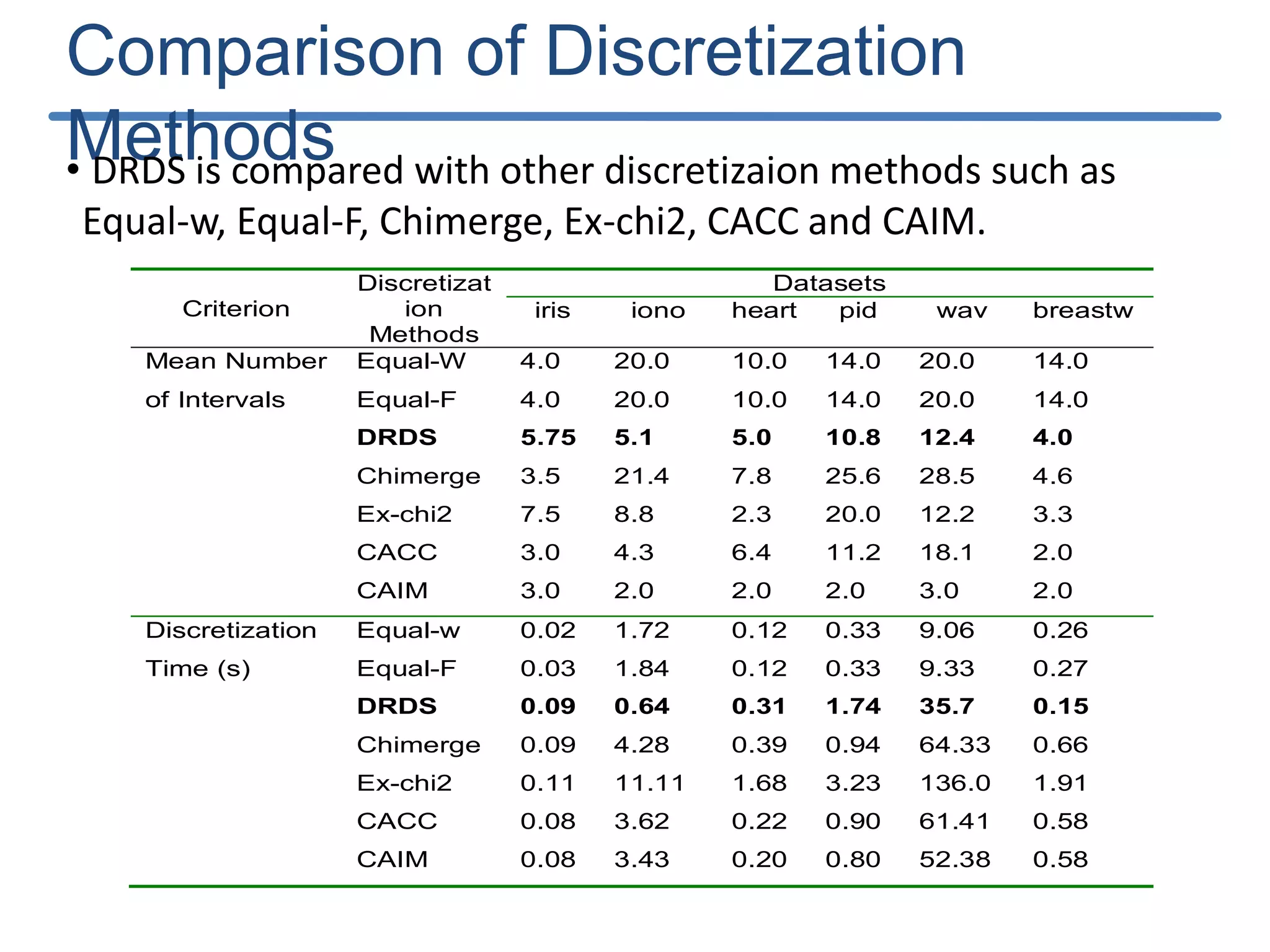
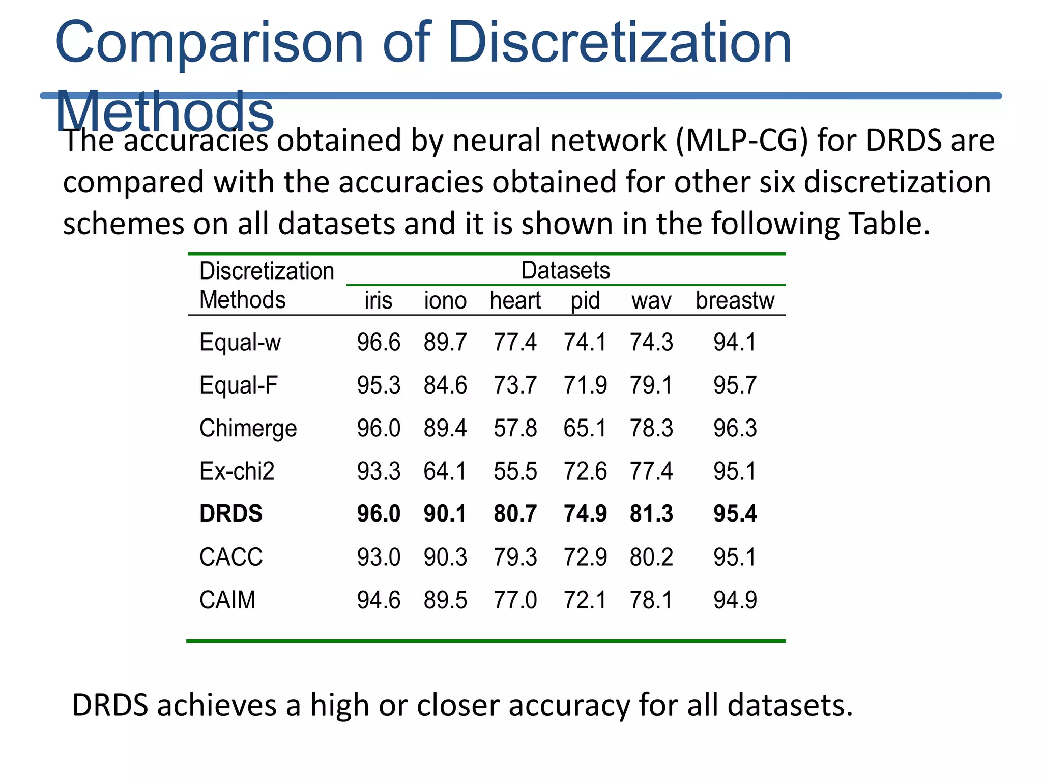
![Results of DRDS Discretization : The results obtained by the DRDS algorithm with the six datasets are shown in Table 2. Classification accuracy: computed using the feed forward neural network with conjugate gradient training (MLP-CG) algorithm[21] with the help of KEEL software [25]. Criterion Datasets iris iono heart pid wav breastw Mean Number of Intervals 5.75 5.1 5.0 10.8 12.4 4.0 Discretization time (s) 0.09 0.64 0.31 1.74 35.7 0.15 Criterion Datasets iris iono heart pid wav breast Topology 23-5-3 175-5-2 65-5-2 87-5-2 495-5-3 36-5-2 Learning time (s) 0.18 0.53 0.59 0.54 34.5 0.34 Training Accuracy (%) 97.9 99.3 96.8 80.4 83.1 99.2 Testing Accuracy (%) 96 90.1 80.7 74.0 81.3 95.4](https://image.slidesharecdn.com/presentationforviva-200509174241/75/Novel-algorithms-for-Knowledge-discovery-from-neural-networks-in-Classification-problems-24-2048.jpg)


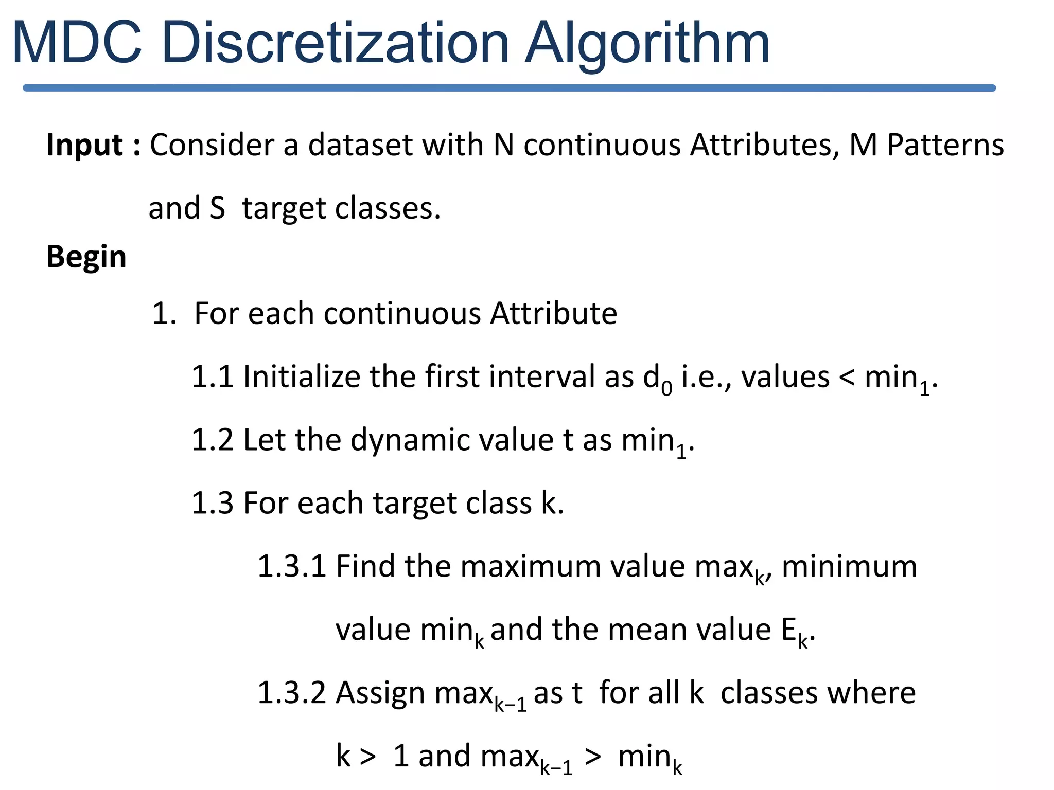
![MDC - Example Age : 10, 8, 24, 43, 12, 61,33 Mean : 27 Interval length : 27-8=19 No. of Intervals : (61-8)/19 ≈ 3 Intervals : [8-27][27-46][46-65] Thermometer coding : for age 12 : 100](https://image.slidesharecdn.com/presentationforviva-200509174241/75/Novel-algorithms-for-Knowledge-discovery-from-neural-networks-in-Classification-problems-65-2048.jpg)
![DRDS - Example Age : 10, 8, 24, 43, 12, 61,33 CD ≈ 0.8 j= 2 [2/3,3/3] jmin=10 Interval length = 2 (10-8) <11 (53/5) Interval length = 4 <11 (53/5) Interval length = 16 No. of Intervals : (61-8)/16 ≈ 4 Intervals : [8-23][24-39][40-55][56-61] After Merging : [8-23][24-61] (if <sqrt(7 ) ≈ 3) Thermometer coding : for age 24 : 01](https://image.slidesharecdn.com/presentationforviva-200509174241/75/Novel-algorithms-for-Knowledge-discovery-from-neural-networks-in-Classification-problems-66-2048.jpg)

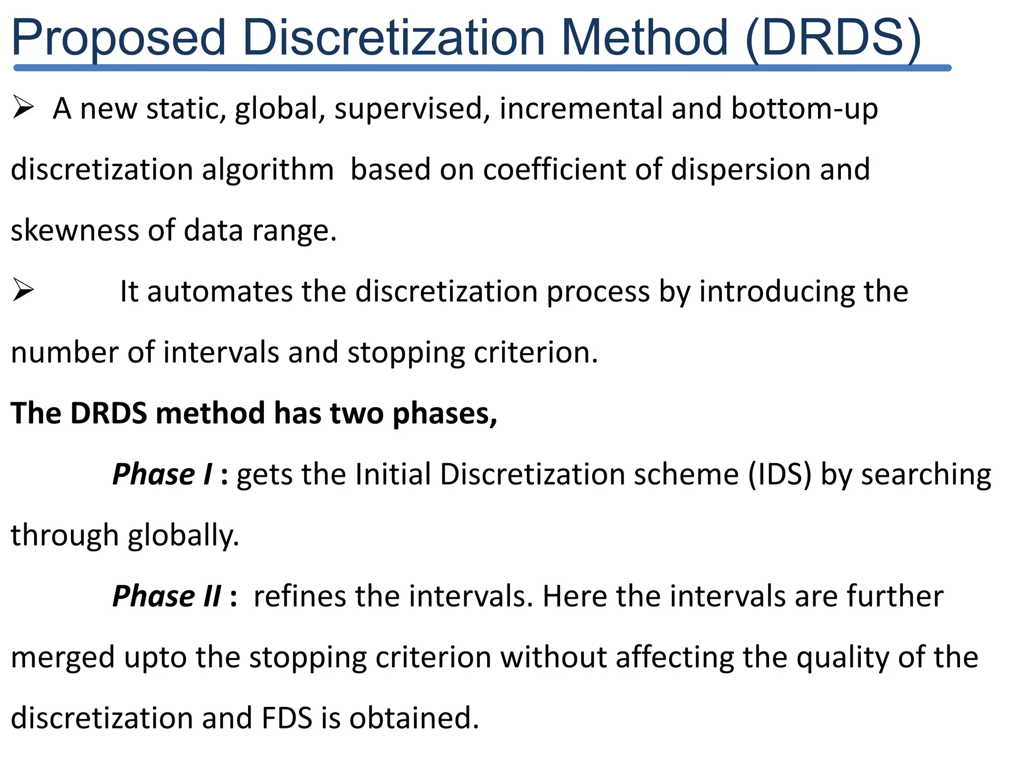
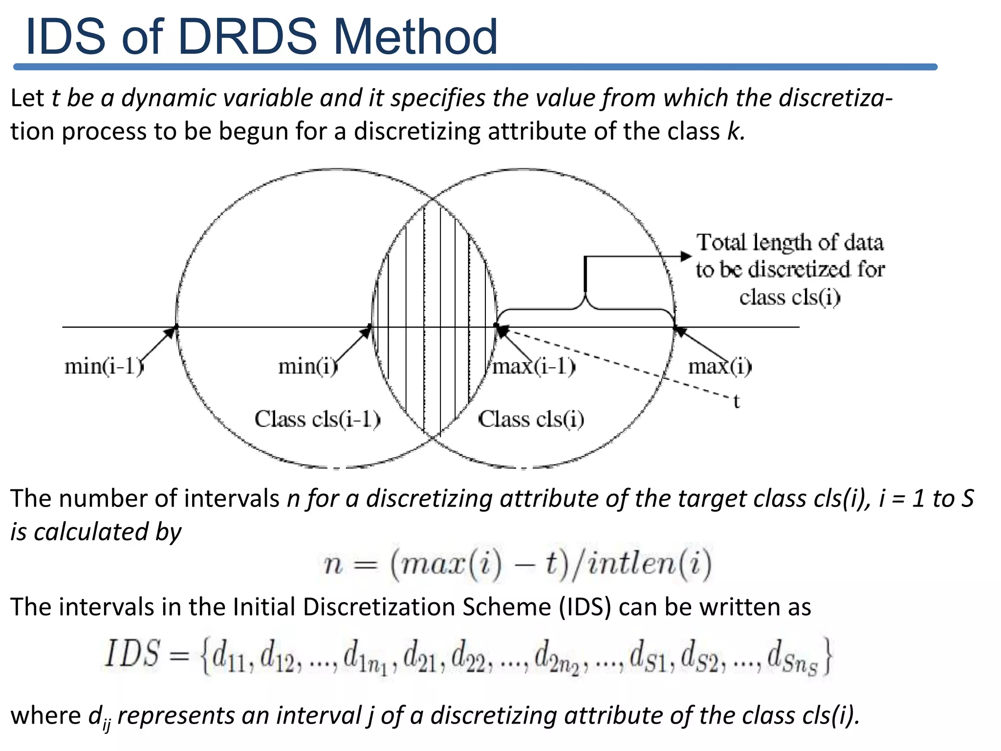
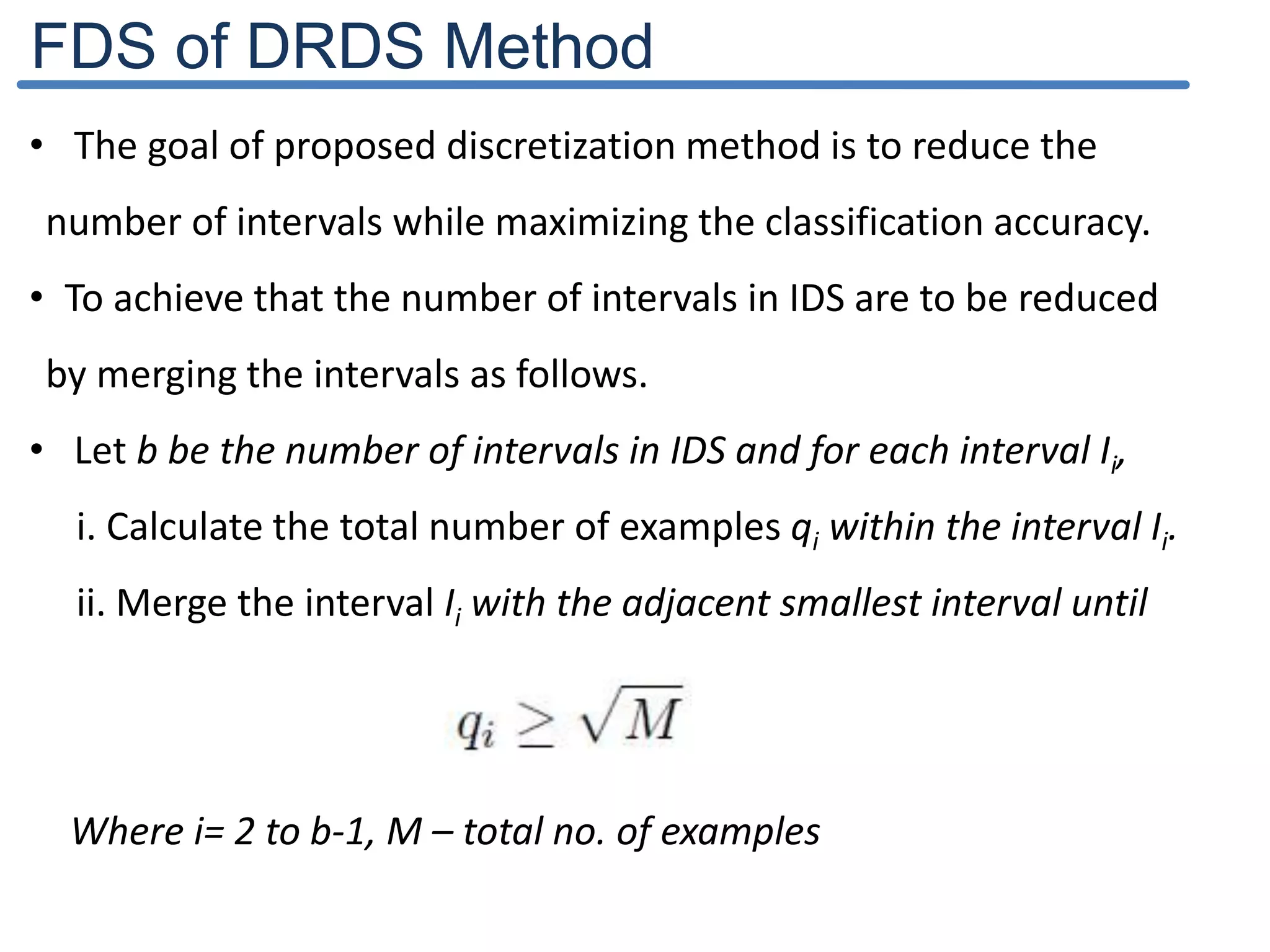
The document describes a new discretization algorithm called DRDS (Discretization based on Range Coefficient of Dispersion and Skewness) for neural networks classifiers. DRDS is a supervised, incremental and bottom-up discretization method that automates the discretization process by introducing the number of intervals and stopping criterion. It has two phases: Phase I generates an Initial Discretization Scheme (IDS) by searching globally, and Phase II refines the intervals by merging them up to a stopping criterion without affecting quality. The algorithm uses range coefficient of dispersion and data skewness to select the best interval length and number of intervals for discretization. Experimental results show DRDS effectively discretizes data for neural network classification.