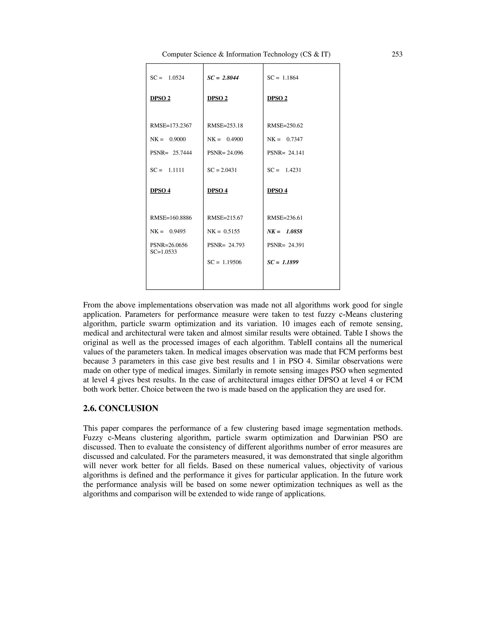
This document evaluates various clustering-based image segmentation techniques, discussing the challenges of consistency and objectivity in segmentation evaluations. It outlines the use of different algorithms, including fuzzy c-means and particle swarm optimization, to enhance segmentation performance. The paper emphasizes the importance of measuring performance parameters and the subjective nature of segmentation, highlighting the dilemma between generality and accuracy.
![David C. Wyld, et al. (Eds): CCSEA, SEA, CLOUD, DKMP, CS & IT 05, pp. 245–254, 2012. © CS & IT-CSCP 2012 DOI : 10.5121/csit.2012.2226 PERFORMANCE ANALYSIS OF CLUSTERING BASED IMAGE SEGMENTATION AND OPTIMIZATION METHODS Jaskirat kaur, Sunil Agrawal and Dr. Renu Vig UIET, Panjab University, Chandigarh jaskiratkaur17@gmail.com ABSTRACT Partitioning of an image into several constituent components is called image segmentation. Myriad algorithms using different methods have been proposed for image segmentation. Many clustering algorithms and optimization techniques are also being used for segmentation of images. A major challenge in segmentation evaluation comes from the fundamental conflict between generality and objectivity. As there is a glut of image segmentation techniques available today, customer who is the real user of these techniques may get obfuscated. In this paper to address the above described problem some image segmentation techniques are evaluated based on their consistency in different applications. Based on the parameters used quantification of different clustering algorithms is done. . KEYWORDS PSO; DPSO; SC; RMSE; NK; PSNR 1. INTRODUCTION Partitioning of an image into several constituent components is called image segmentation. Segmentation is an important part of practically and automated image recognition systems, because it at this moment extracts the intensity objects, for further processing such as description or recognition [1]. It is widely used in exploratory pattern-analysis, grouping, decision making, machine learning situations, including data mining, document retrieval and pattern classification [2]. In many such above mentioned cases, there is little a priori information available about the data and we need to make as many assumptions as possible. Under all these restrictions clustering methodology is particularly appropriate for the exploration of interrelationship among the data points to make an assessment of their structure [2]. Today many data clustering algorithms are being used for segmenting images. They are termed as unsupervised methods for segmentation of images. In such techniques, image is separated into a set of disjoint regions with each region associated with one of the finite number of classes that are characterized by distinct parameters [3]. Therefore till date many types of segmentation techniques have been developed and many data clustering techniques are being used for segmentation of images [4]. A potential problem for a measure of consistency between different segmentations available is that there is no unique segmentation of an image. For example two people may segment an image differently because they either perceive the scene differently, or they segment at different](https://image.slidesharecdn.com/csit2226-180131090745/75/PERFORMANCE-ANALYSIS-OF-CLUSTERING-BASED-IMAGE-SEGMENTATION-AND-OPTIMIZATION-METHODS-1-2048.jpg)
![246 Computer Science & Information Technology (CS & IT) granularities. If two different segmentations arise from different perceptual organizations of the scene, then it is fair to declare the segmentations inconsistent [5]. A major challenge in segmentation evaluation comes from the fundamental conflict between generality and objectivity. For general-purpose segmentation, segmentation accuracy may not be well defined, while embedding the evaluation in a specific application, the evaluation results may not be extensible to other applications. Reliable segmentation performance evaluation for quantitatively positioning image segmentation is extremely important. In many prior works, segmentation performance is evaluated by subjectively or objectively judging several sample images. Such evaluations lack statistical meanings and may not be generalized to other images and applications [4]. As there is a glut of image segmentation techniques available today, customer who is the real user of these techniques may get obfuscated. In this paper to address the above described problem performance analysis is carried out to classify and quantify different clustering algorithms based on their consistency in different applications. This paper also describes the various performance parameters on which consistency will be measured [3]. The rest of the paper is organized as follows: Section II discusses various clustering based image segmentation techniques. Section III describes parameters used to measure consistency. Experimental implementation and results are shown in Section IV. Section V concludes the paper. 2. CLUSTERING BASED IMAGE SEGMENTATION METHODS Extracting information from an image is referred to as image analysis. It is one of the preliminary steps in pattern recognition systems. Each region of the image is made up of set of pixels. Partitioning an image into several disjoint segments is termed as image segmentation. It simplifies and changes the representation of an image, transferring an image into something more meaningful and easier to analyze. Typically it is used to locate objects of interest and boundaries like lines, and curves in an image [1]. Segmentation algorithms are based on two basic properties of an image intensity value: discontinuity and similarity. To study discontinuities in an image we divide image based on the abrupt changes in intensity such as edges. Mathematically the regions we obtain after partitioning an image is considered to be homogeneous with respect to some image property of interest. Image property can be intensity, color, or texture. If ܫ = {ݔ, ݅ = 1 … ܰ, ݆ = 1 … ܰ} (1) is the input image with ܰ rows and ܰ columns and measurement value ݔ at pixel (݅, ݆), then the segmentation can be expressed as ݈ = {ܵଵ, … . , ܵ } with the ݈௧ segment ܵ = {൫݅భ , ݆భ ൯, … , ቀ݅ಿభ , ݆ಿభ ቁ} (2) consisting of a connected subset of the pixel coordinates. No two segments share any pixel locations and the union of all the segments covers the entire image. An image may contain more than one object and segmenting the image in line with object features in order to extract meaningful object has become a challenge for researchers in the field. Segmentation can be achieved in a more efficient manner through clustering.](https://image.slidesharecdn.com/csit2226-180131090745/75/PERFORMANCE-ANALYSIS-OF-CLUSTERING-BASED-IMAGE-SEGMENTATION-AND-OPTIMIZATION-METHODS-2-2048.jpg)
![Computer Science & Information Technology (CS & IT) 247 Clustering is an interesting approach for finding similarities in data and putting similar data into groups. Cluster partitions data set into several groups such that the similarity within a group is larger than that among the groups. Clustering algorithms are used extensively not only to organize and categorize data, but are also useful for data compression [6]. The segmentation of images presented to an image analysis system is critically dependent on the scene to be sensed, the imaging geometry, configuration, and sensor used to convert the scene into a digital image, and ultimately the desired output of the system [6]. The applicability of clustering methodology to the image segmentation problem was recognized over three decades ago, and the paradigms underlying the initial pioneering efforts are still in use today. It defines feature vectors at every image location called as pixel component of both functions of image intensity and functions of pixel location itself. Figure1. Feature representation for clustering The basic idea of assigning pixel values is depicted in figure 1. In the above figure image measurements and positions are transformed to features. Also clusters in feature space correspond to image segments [6]. Good objectivity means that all the test images should have an unambiguous segmentation so that segmentation evaluation can be conducted objectively. Good generality means that test images should have a large variety so that the evaluation results can be extended to other images and applications. There always exists a well known dilemma between objectivity and generality in segmentation evaluation [4]. There is no such unique clustering technique which can segment all types of images uniquely and unambiguously. 2.1. Fuzzy c-means Clustering Algorithm In fuzzy clustering, the image pixel values can belong to more than one cluster, and associated with each of the points are membership grades that indicate the degree to which the data points belong to different clusters [7]. The input to FCM algorithm is, ݊ × ݉ matrix where ݊ is the number of data and ݉ is the number of parameters, ܿ the number of clusters, the assumption partition matrix ܷ, and the convergence value .ܧ The assumption partition matrix have ܿ number of rows, ݊ number of columns, and contain values 0 to 1. The sum of every column has to be 1. The first step in FCM algorithm is to calculate the cluster centers. This is a matrix ݒ of dimension ܿ rows with ݉ columns. The second step is to calculate the distance matrix .ܦ The distance matrix constitutes the Euclidean distance between every pixel and every cluster center. This is matrix with ܿ rows and ݊ columns. From the distance matrix the partition matrix ܷ is calculated. If the difference between the initial partition matrix and the calculated partition matrix is greater than the convergence value then the entire process from calculating the cluster centers to the final](https://image.slidesharecdn.com/csit2226-180131090745/75/PERFORMANCE-ANALYSIS-OF-CLUSTERING-BASED-IMAGE-SEGMENTATION-AND-OPTIMIZATION-METHODS-3-2048.jpg)
![248 Computer Science & Information Technology (CS & IT) partition matrix. The final partition matrix is taken and is used for reconstructing the image. Fuzzy c-Means function is taken as ܬ(ܷ, ܻ) = ∑ ∑ (ݑ) ܧ(ݔ) ୀଵ ୀଵ (3) Where Ω = { ݔ | k € [1, n]} is a training set containing ݊ unlabeled symbols ; Y = {ݕ | j € [1,c]}} is the set of centers of clusters; ܧ(ݔ) is a dissimilarity measure between the sample ݔ and the cluster ݕ of a specific cluster j; ܷ = [ݑ] is the ܿ × ݊ fuzzy c partition matrix, containing the membership values of all samples in all clusters; ݉ € (1, ∞) is a control parameter of fuzziness. The clustering problem can be defined as the minimization of ܬ with respect to Y, under the probabilistic constraint: ∑ ൫ݑ൯ = 1 ୀଵ (4) The FCM algorithm consists in the iteration of the following formulas: for all j ݕ = ∑ (௨ೕೖ) ௫ೖ ೖసభ ∑ (௨ೕೖ) ೖసభ (5) And ݑ =ቂ ((∑ ( ாೕ (௫ೖ ) ா (௫ೖ ) ) మ షభ) ୀଵ ቃ ିଵ ݂݅ ܧ(ݔ) > 0 ∀݆, ݇ (6) Where in the case of Euclidean space: ܧ = |หݔ − ݕห|ଶ (7) If ݉ is chosen to be equal to be 1 the FCM function ܬ , equation 3 reduces to the expectation of the global error denoted as <.>ܧ < ܧ ≥ ∑ ∑ ݑܧ ୀଵ ୀଵ (ݔ) (8) 2.2. Particle Swarm Optimisation PSO has been originally introduced in terms of social behavior of particles. The individuals, called particles are made to flow through the multidimensional search space. Each particle then tests a possible solution to the multidimensional problem as it keeps on moving through the problem space. The movement of the particles is influenced by two factors, the particle's best solution (pbest) and the global best solution found by all the particles (gbest), which influence the particle's velocity through the search space by creating an attractive force [9]. As a result, the particle interacts with all neighbors and stores optimal location information in its memory. After each iteration the pbest and gbest are updated respectively if a more optimal solution is found by the particle or population. This process is continued iteratively until either the desired result is achieved. The PSO formulae defines each particle in the D- dimensional space as xi =(xi1 ,xi2 , ,xiD), where the subscript i represents the particle number and the second subscript is the dimension. The memory of the previous best position (pbest) is represented as Pi = ( pi1, pi2, , piD) and a velocity along each dimension as vi = (vi1, vi2, , viD) . After each iteration, the velocity term is updated. The](https://image.slidesharecdn.com/csit2226-180131090745/75/PERFORMANCE-ANALYSIS-OF-CLUSTERING-BASED-IMAGE-SEGMENTATION-AND-OPTIMIZATION-METHODS-4-2048.jpg)
![Computer Science & Information Technology (CS & IT) 249 particle's motion is influenced by its own best position Pi, as well as the global best position Pg (gbest),[8]. The velocity is updated by vij (t +1) = wvij (t)+c1r1(pij(t)−xij(t))+c2r2(pgj(t)−xij(t)) (9) And the position is updated by xij (t +1) = xij(t) +vij(t +1) (10) Constants c1, c2 determine the relative influence of the pbest and gbest and they are set to same value. The memory of the PSO is controlled by w [13]. r1, r2 are randomly generated value between 0 and 1. The PSO is usually executed with repeated application of (9) and (10) until a specified number of iterations have been exceeded. Alternatively, the algorithm also can he terminated when the velocity updates are close to zero over a number of iterations. 2.3. Darwinian Particle Swarm Optimisation Darwinian PSO, in which many swarms of test solutions may exist at any time. Each swarm individually performs just like an ordinary PSO algorithm with some rules governing the collection of swarms that are designed to simulate natural selection [10]. The selection process implemented is a selection of swarms within a constantly changing collection of swarms. The basic assumptions made to implement Darwinian PSO are: • The longer a swarm lives, the more chance it has of possessing offspring. This is achieved by giving each swarm a constant, small chance of spawning a new swarm. • A swarm will have its life-time extended (be rewarded) by finding a more fit state. • A swarm will have its life-time reduced (be punished) for failing to find a more fit state. Steps of Darwinian PSO 1) Particle and swarm initialization Each PSO particle is an array of N numbers; the array could contain a binary string [11]. The choice of the domain of the particle array elements, xi as well as the encoding of the test solution as an array of numbers is motivated by the particular optimization problem. The discussion of these details is therefore deferred until thetest problems are discussed. Each dimension of each particle is randomly initialized on an appropriate range xmin ≤ xi≤ xmax. The velocities are also randomly initialized on a range, vmin ≤ vi≤ vmax , that allows particles to traverse a significant fraction of the range of xi in a single iteration when moving at vi = vmax . The algorithm says to evolve an individual swarm, the fitness of all of the particles in the swarm are evaluated. The neighborhood and individual best positions of each of the particles are updated. The swarm spawns a new particle if a new global best fitness is found. A particle is deleted if the swarm has failed to find a more fit state in an allotted number of steps. 2) Condition for deleting a swarm A swarm's particle population, m is bounded such that, mmin ≤ m≤ mmax . When a swarm's population falls below mmin , the swarm is deleted. 3) Condition for deleting a particle](https://image.slidesharecdn.com/csit2226-180131090745/75/PERFORMANCE-ANALYSIS-OF-CLUSTERING-BASED-IMAGE-SEGMENTATION-AND-OPTIMIZATION-METHODS-5-2048.jpg)
![250 Computer Science & Information Technology (CS & IT) The worst performing particle in the swarm is deleted using the following algorithm. The number of times a swarm is evolved without finding an improved fitness is tracked with a search counter, SC. If the swarm's search counter exceeds a maximum critical threshold, SCmax, a particle is deleted from the swarm. When a swarm is created, its search counter is set to zero. When a particle is deleted, the swarm's search counter is reset not to zero but to a value approaching SCmax as the time during which the swarm makes no improvement in fitness increases. The purpose of this reduction in tolerance for stagnation is to try to maintain a collection of swarms that are actively improving. If Nkill is the number of particles deleted from the swarm over a period in which there is no improvement in fitness, then the reset value of the search counter is chosen to be ܵܥ(ܰ) = ܵܥ ௫ ቂ1 − ଵ ேೖାଵ ቃ (11) 4) Condition for spawning particles and swarms At each step of the algorithm, each swarm may spawn a new swarm. To be able to spawn a new swarm, an existing swarm must have Nkill = 0. If this condition is met and the maximum number of swarms will not be exceeded, the swarm spawns a new swarm with probability p = f / Ns , where f is a uniform random number [0,1] and Ns is the number of swarms. The purpose of the factor of 1/ Ns is to suppress swarm creation when there are large numbers of swarms in existence. When a swarm spawns a new swarm, the spawning swarm (parent) is unaffected. To form the spawned (child) swarm, half of the particles in the child are randomly selected from the parent swarm and the other half are randomly selected from a random member of the swarm collection (mate). The spawned or child swarm may inherit other attributes from either parent or mate as necessary to design experimentation for the Darwinian PSO algorithm. A particle is spawned whenever a swarm achieves a new global best fitness. 3. PARAMETERS TO MEASURE CONSISTENCY 1) Structural Content (SC) SC = ∑ ∑ (,)మಿ ೖసభ ಾ ೕసభ ∑ ∑ (,)మಿ ೖసభ ಾ ೕసభ (12) The large value of structural content means that image is of poor quality [3]. 2) Peak signal to noise ratio (PSNR) PSNR = 10. ݈݃ଵ ۏ ێ ێ ۍ ୫ୟ୶ ((௫,௬))మ భ ೣ. ∑ ∑ [ೝ(ೣ,)]మషభ బ ೣషభ బ ∑ ∑ [ೝ(ೣ,)ష(ೣ,)]మషభ బ ೣషభ బ ൩ ے ۑ ۑ ې (13) The above equation calculates PSNR in decibels. The small value of PSNR means the image is of poor quality [3].](https://image.slidesharecdn.com/csit2226-180131090745/75/PERFORMANCE-ANALYSIS-OF-CLUSTERING-BASED-IMAGE-SEGMENTATION-AND-OPTIMIZATION-METHODS-6-2048.jpg)
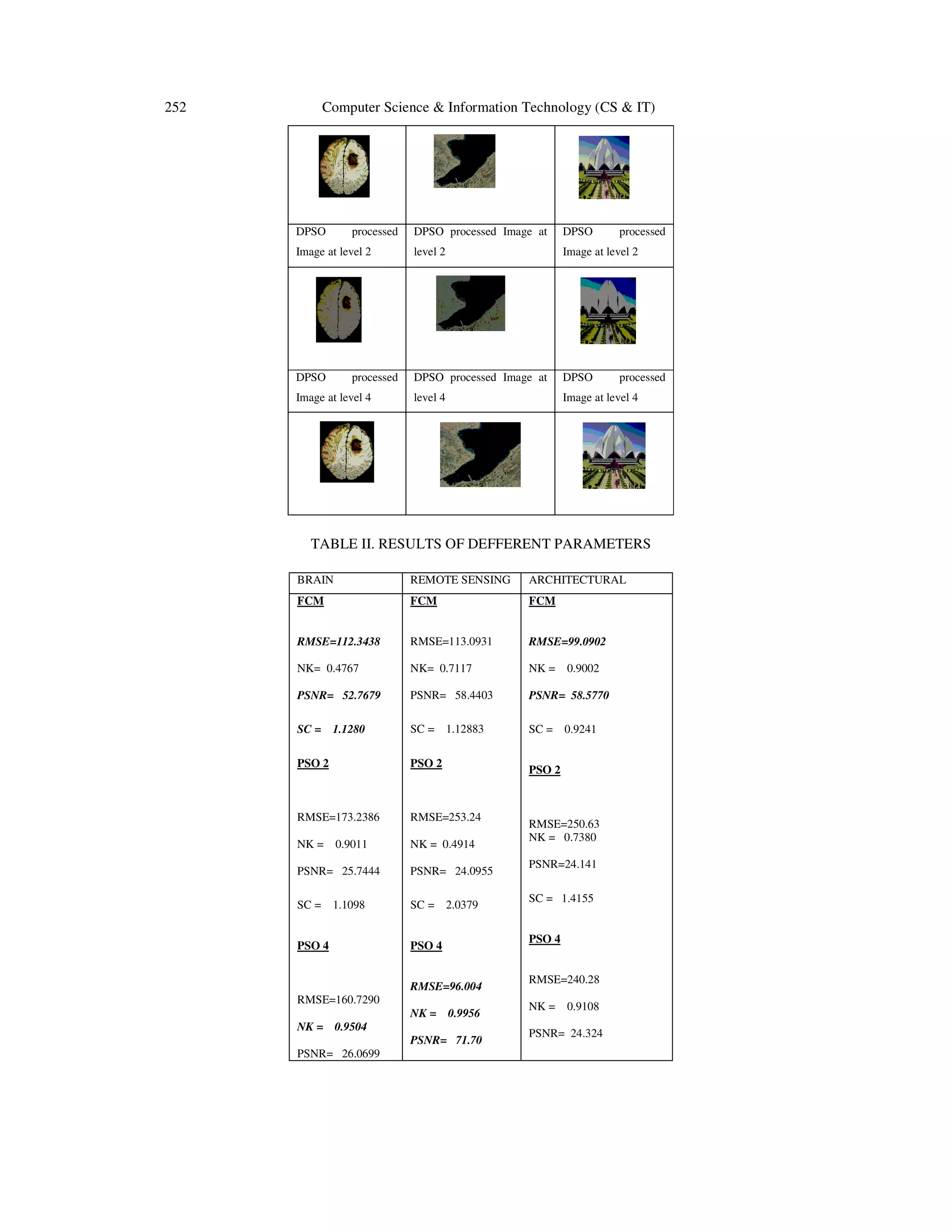
![Computer Science & Information Technology (CS & IT) 251 3) Normalized Correlation Coefficient (NK) NK = ∑ ∑ [(,)(,)]ಿ ೖసభ ಾ ೕసభ ∑ ∑ [(,)మಿ ೖసభ ಾ ೕసభ ] (14) 4) Root mean square error (RMSE) RMSE = ඨ ଵ ೣ. ቈ ∑ ∑ [(௫,௬)]మ షభ బ ೣషభ బ ∑ ∑ [(௫,௬)ି௧(௫,௬)]మ షభ బ ೣషభ బ (15) This is the simplest image quality measurement. The large value of RMSE means the image is of poor quality. RMSE and PSNR compares the input image r(x,y) with the output image t(x,y). 4. EXPERIMENTAL ANALYSIS AND RESULTS In this section different clustering based image segmentation methods are applied to images from different fields and the algorithms were tested for consistency for each application. One image from each section is presented over here and the values of parameters are calculated. Numerical values define the objectivity of different clustering algorithms. TABLE I. IMAGES FROM DIFFERENT FIELDS AND THE PROCESSED OUTPUTS Original Brain tumour image Original Remote sensing image Original Architectural image FCM processed Image FCM processed Image FCM processed Image PSO processed Image at level 2 PSO processed Image at level 2 PSO processed Image at level 2 PSO processed Image at level 4 PSO processed Image at level 4 PSO processed Image at level 4 Segmentation using FCM](https://image.slidesharecdn.com/csit2226-180131090745/75/PERFORMANCE-ANALYSIS-OF-CLUSTERING-BASED-IMAGE-SEGMENTATION-AND-OPTIMIZATION-METHODS-7-2048.jpg)
![254 Computer Science & Information Technology (CS & IT) REFERENCES [1] B.Sowmya and B.Sheelarani, “Colour Image Segmentation Using Soft Computing techniques,” International Journal of Soft Computing Applications, Issue-4(2009), pp.69-80. [2] Shilpa Agarwal, Sweta Madasu, Madasu Hanmandlu and, Shantaram Vasikarla, “A Comparison of some Clustering Techniques via Color Segmentation,” International Conference on Information Technology: Coding and Computing (ITCC’05), 0-7695-2315-3/05, IEEE. [3] R.Harikumar, B. Vinoth Kumar and, G.Karthick and I.N. Sneddon, “Performance Analysis for Quality measures Using K means Clustering and EM models in segmentation of medical Images,” International Journal of Soft computing and Engineering, vol. 1, Issue-6, pp.74-80, January 2012. [4] Feng Ge, Song Wang and, Tiecheng Liu, “New Benchmark for image segmentation evaluation,” Journal of Soft Electronic Imaging, 16(3), 033011, pp.033011-1-16, Jul-sep 2007 [5] Alina Doringa, Gabriel Mihai, Liana Stanescu, Dumitru Dan Burdesce, “Comparison of Two Image Segmentation Algorithms,” Second International Conferences on Advances in Multimedia, 978-0- 7695-4068-9/10, 2010 IEEE. [6] A.K. Jain, M.N. Murty and, P.J. Flynn, “Data clustering: A Review,” ACM computing Surveys, vol.31, No. 3, September 1999 [7] Songcan Chen, Daoqiang Zhang, “Robust image segmentation usinf FCM with spatial constraints based on new kernel – induced distance measure” International Journal of Soft Computing Apllications, ISSN:1453-2277, Issue 4(2009), pp.69-80. [8] J. Zeng, J. Jie, Z. Cui, "Particle swarm optimization algorithm," Beijing Science Press. 2004. [9] Li Wang, Yushu Liu and Xinxin Zhao, Yuanqing Xu, “Particle swarm optimization for Fuzzy c- Means clustering”, Proceedings of 6th world congress on intelligent control and automation, 1-4244- 0332-4,Dalian, China, 2006,pp 6055-6058. [10] Jason Tillett, T.M. Rao, Ferat Sahin and Raghuveer Rao, “Darwinian particle swarm optimization,” University of Rochester, Rochester, NY USA. [11] Kennedy, J. and R.C. Eberhart, “ A discrete binary version of the particle swarm algorithm. in Systems”, Man, and Cybernetics. 1997. Piscataway, NJ: IEEE Service Center. [12] Y. shi, R. Eberhart, "A modified particle swarm optimizer," in Proc. of IEEE Intl. Conf. on Computational Intelligence, pp. 69-73, 1998 [13] Google Images. Retrieved in febraury, 2012 from http://www.google.ca/imghp?hl=en&tab=wi](https://image.slidesharecdn.com/csit2226-180131090745/75/PERFORMANCE-ANALYSIS-OF-CLUSTERING-BASED-IMAGE-SEGMENTATION-AND-OPTIMIZATION-METHODS-10-2048.jpg)