Downloaded 1,390 times

![3.6 Sensor Protocol for Information via Negotiation family of protocols for information via negotiation (SPIN) is proposed in [5]. SPIN uses negotiation and resources and adaption to address the deficiencies of flooding. Negotiation reduces overlap and implosion, and a threshold based resource-aware operation is used to prolong network lifetime. Meta-data, or data describing data, is transmitted instead of row data. This requires fewer bytes and can be in an application-specific format. SPIN has three types of messages: ADV,REQ, and DATA. A sensor node broadcasts an ADV containing meta-data describing actual data. If a neighbor is interested in the data , it sends REQ for the data. Then the sensor node sends the actual DATA to the neighbor. The neighbor again sends ADVs to its neighbors and this process continues to disseminate the data throughout the network. the simple version is shown in figure. Figure 3.3: Sensor Protocol for Information via Negotiation SPIN is based on data-centric routing, where the nodes advertise the available data through an ADV and wait for requests from interested nodes. SPIN-2 expands on SPIN, using an energy or resource threshold to reduce participation. A node may participate in the ADV-REQ-DATA handshake only if it has sufficient resources above a threshold. 11](https://image.slidesharecdn.com/wsn-120411080136-phpapp01/75/Routing-Protocols-for-Wireless-Sensor-Networks-17-2048.jpg)


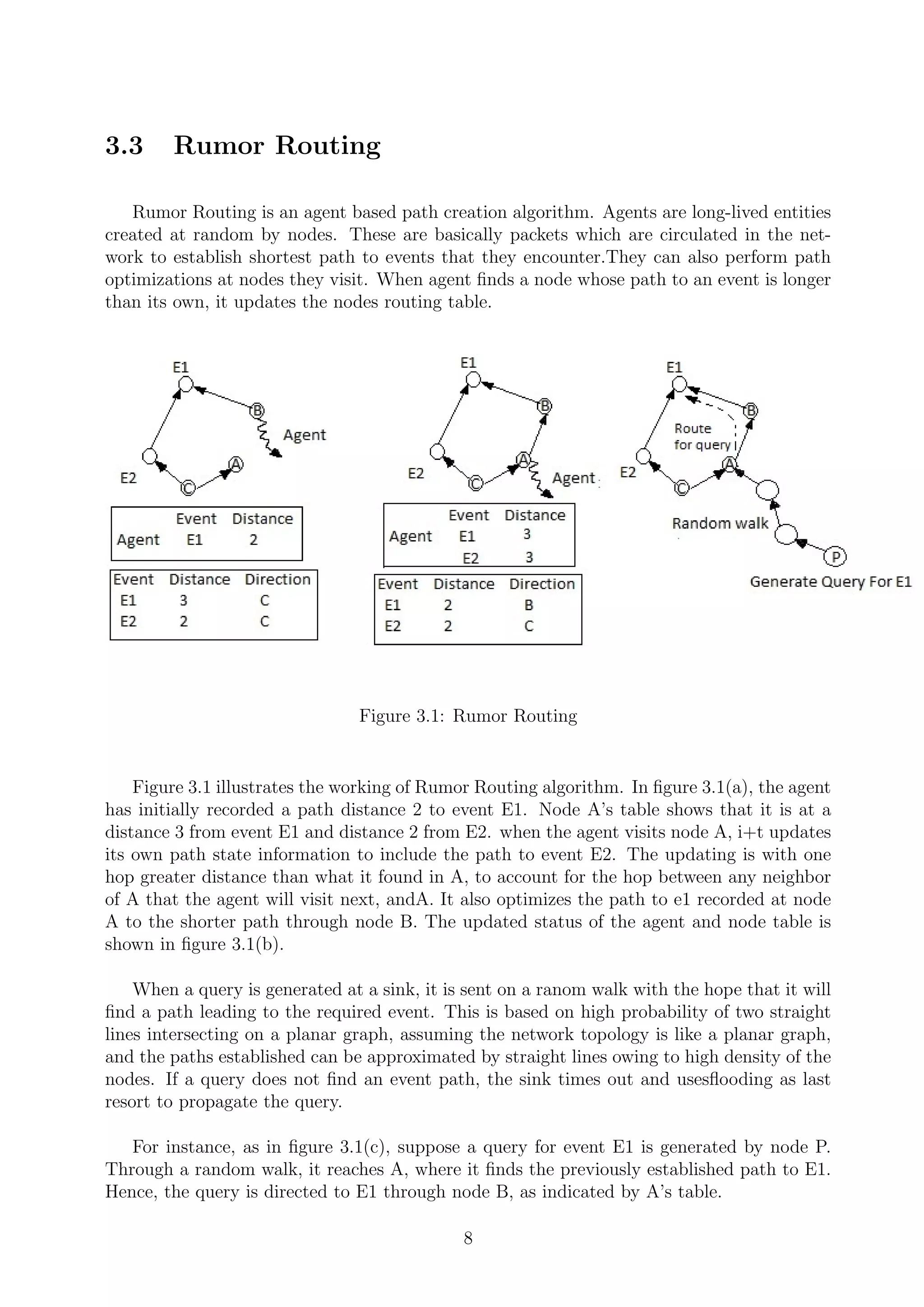
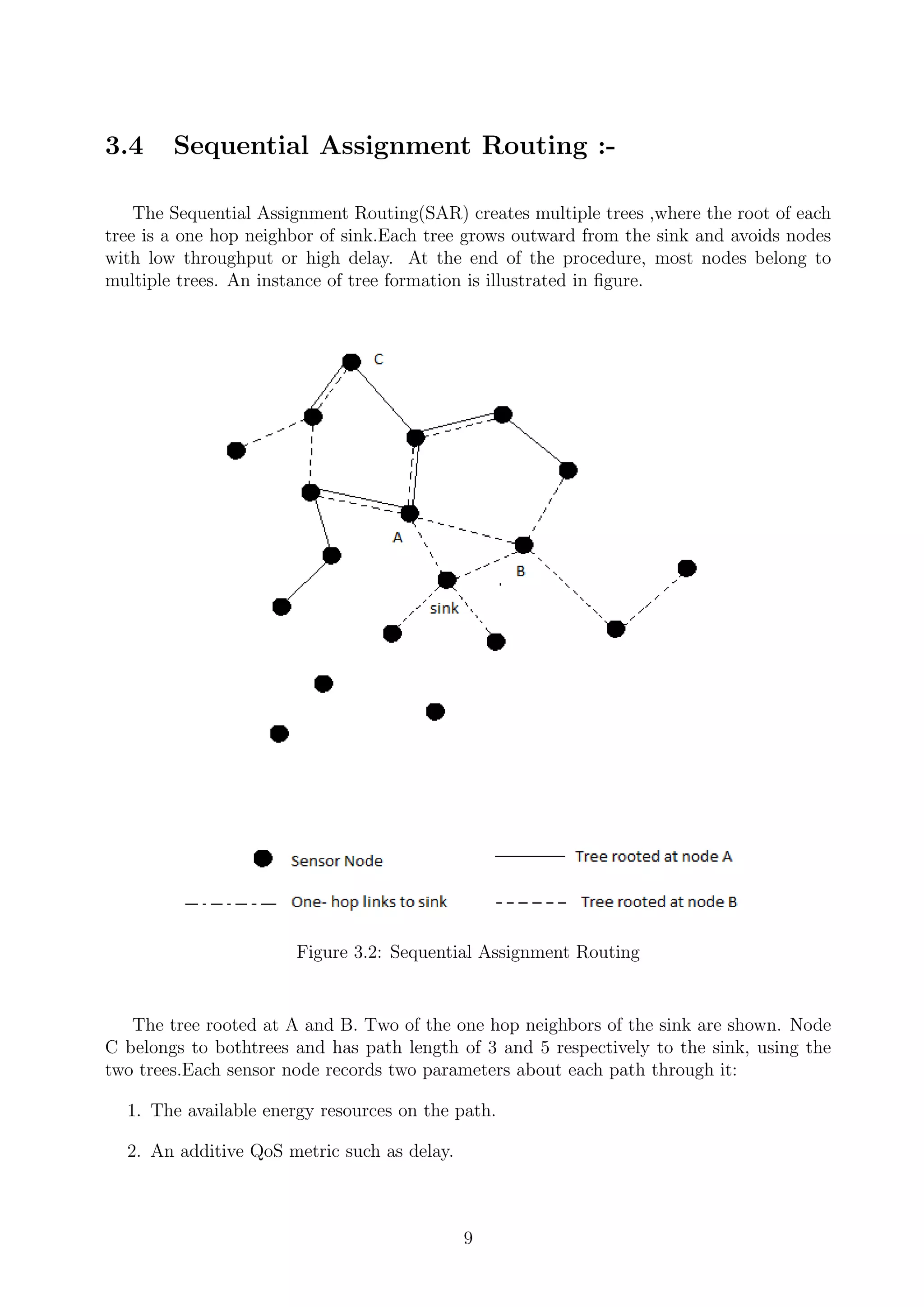
The document discusses various data dissemination protocols in wireless sensor networks. It describes flooding, gossiping, rumor routing, sequential assignment routing, direct diffusion, SPIN, and geographic hash table protocols. Flooding broadcasts packets to all neighbors, causing implosion and resource blindness issues. Gossiping sends packets randomly to one neighbor to avoid implosion. Rumor routing and direct diffusion use flooding initially and then optimize routing. SPIN uses data advertisements before transmission. Geographic hash table hashes node locations to optimize routing.
Overview of the seminar topic focusing on power-aware routing protocols in wireless sensor networks (WSNs) for a Bachelor of Technology degree.
Certification of the seminar by professors, affirming the originality and supervision in the work presented on power-aware routing.
Discussion of advancements in micro-sensor devices and various routing protocols for WSNs focusing on data dissemination and comparisons.
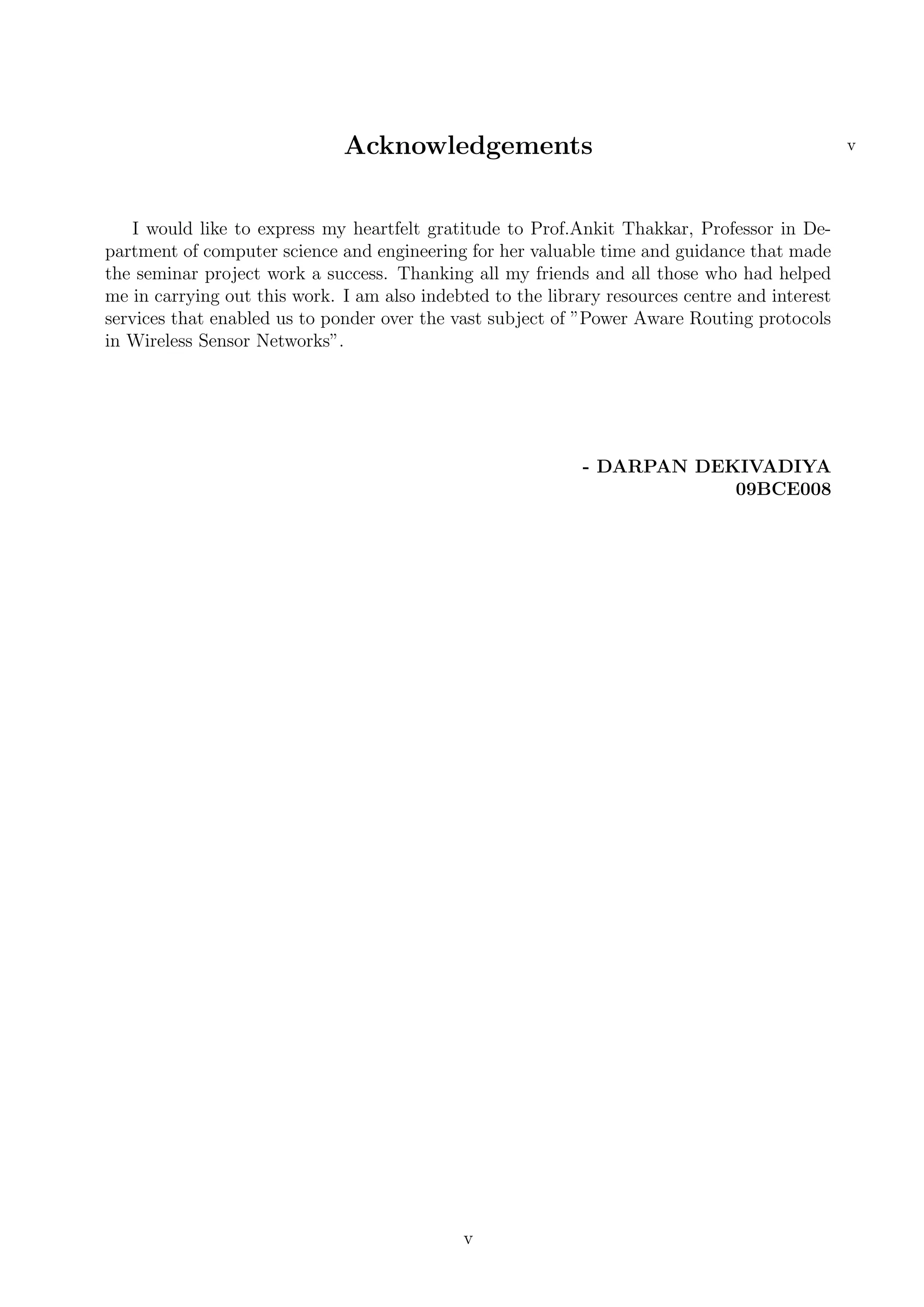
Expression of gratitude from Darpan Dekivadiya to professors and friends for support during the seminar project.
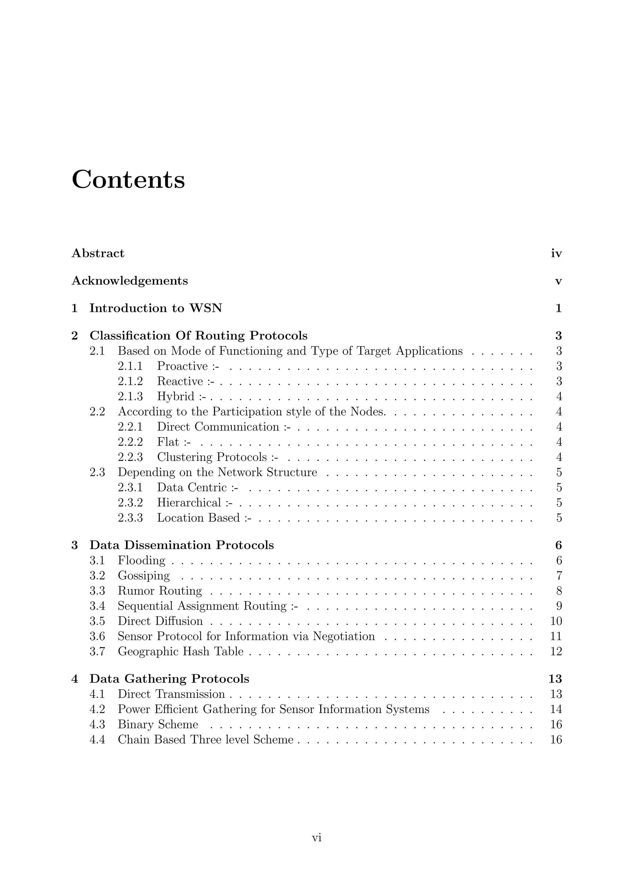
Outline of the seminar report including sections on Introduction, Classification of Routing Protocols, Data Dissemination and Gathering Protocols.
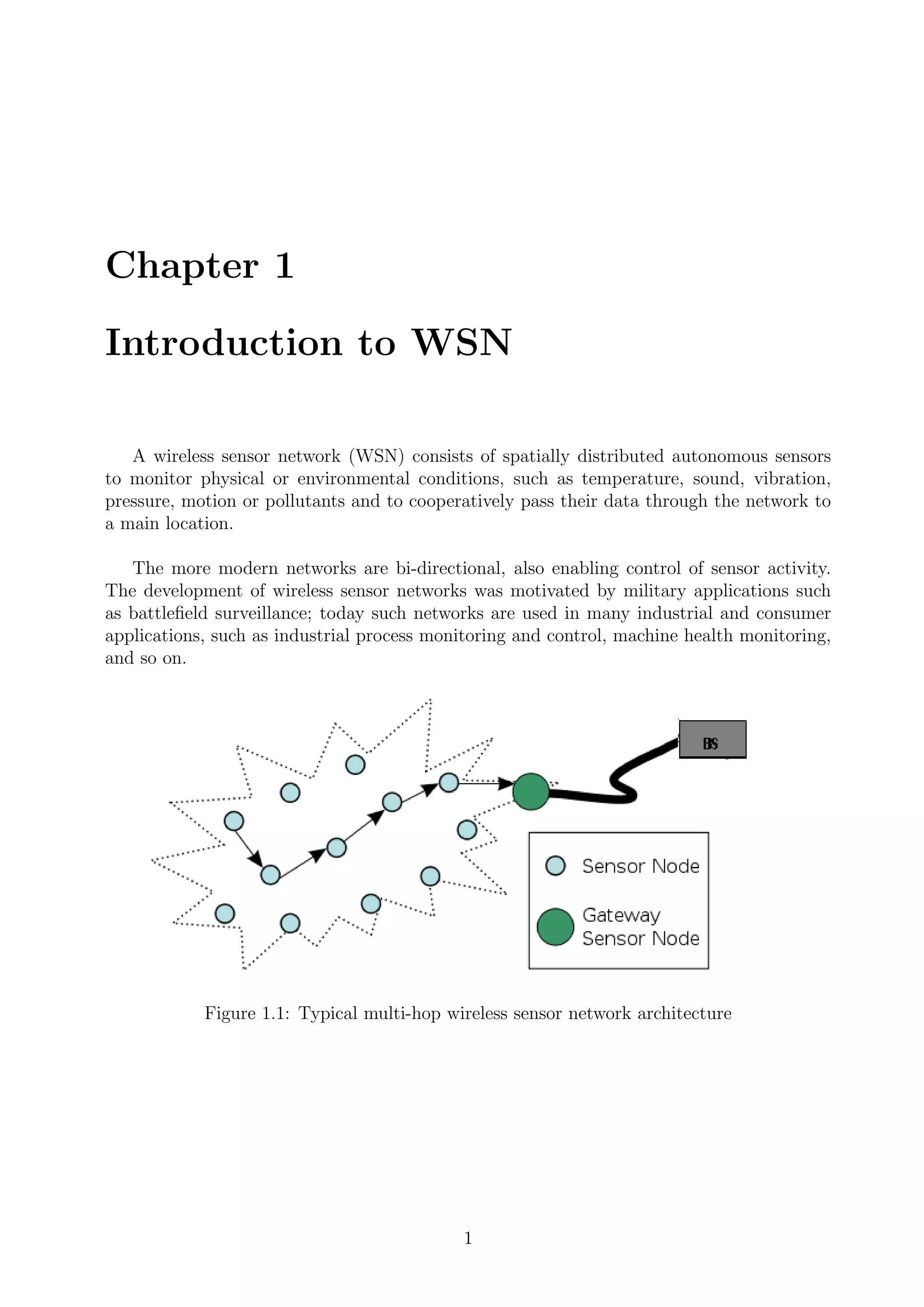
Description of WSNs, their structure, and components, including nodes, sensors, and network topologies used for monitoring conditions.
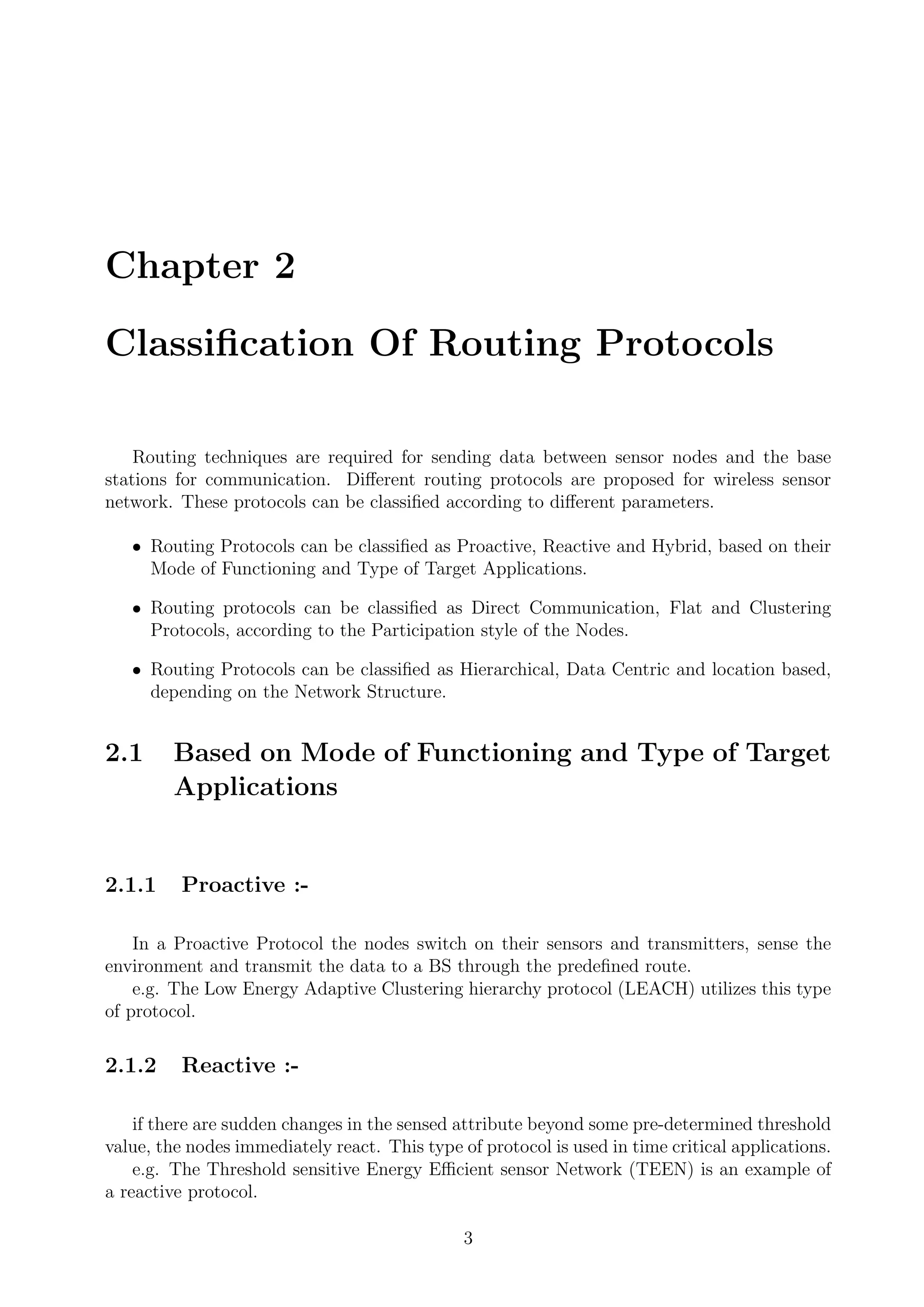
Detailed classifications of routing protocols in WSNs based on different parameters, including proactive, reactive, and hybrid protocols.
Introduction to data dissemination methods in WSNs, emphasizing how data is routed to sinks from sensor nodes.
Explanation of flooding and gossiping methods for data transmission, including their advantages and limitations in energy efficiency.
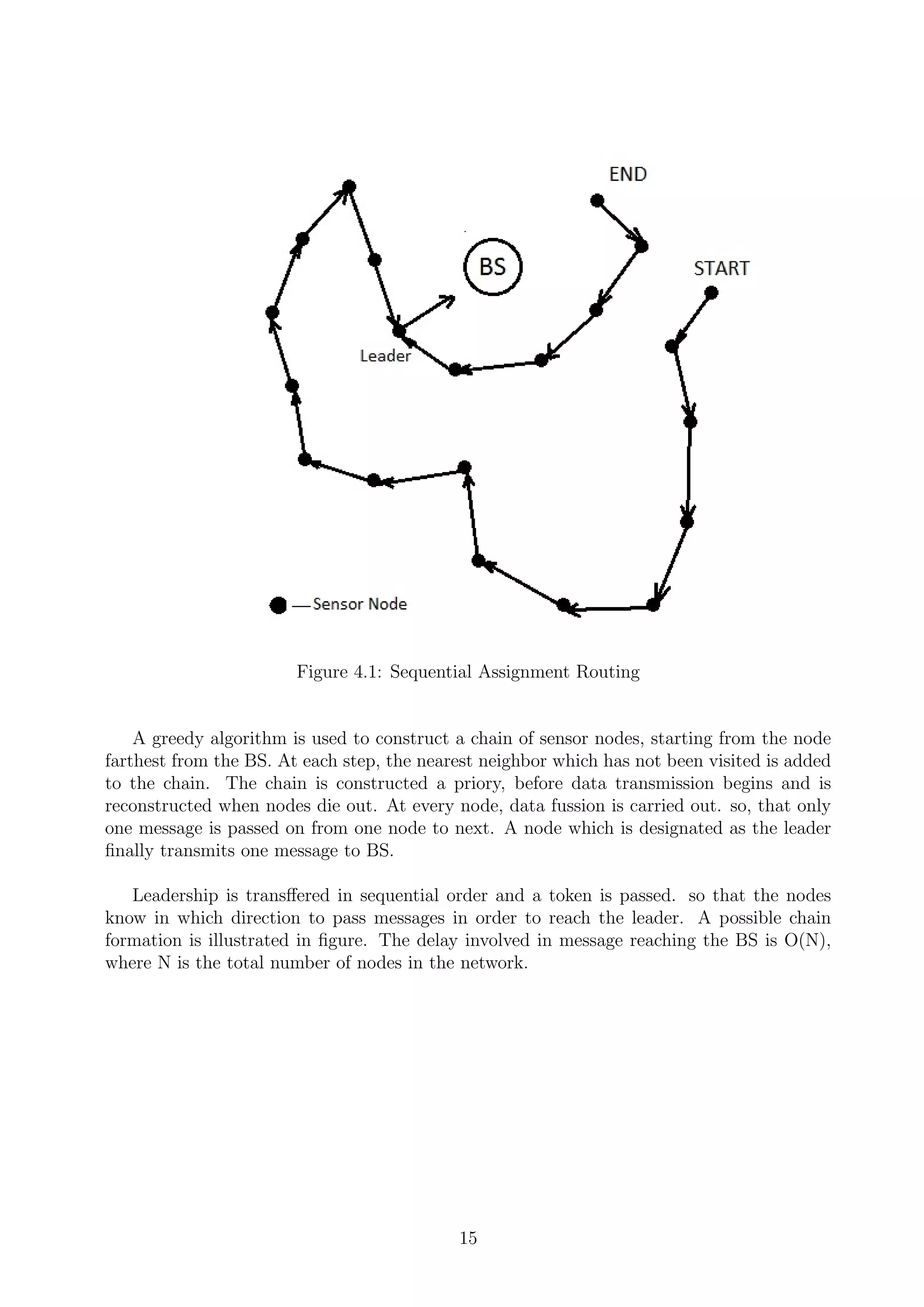
Details on Sequential Assignment Routing (SAR) and Direct Diffusion protocols, focusing on energy efficiency and data gathering.
Description of SPIN protocols that utilize negotiation to efficiently disseminate information within WSNs.
Explanation of the Geographic Hash Table and its role in data-centric storage and routing within sensor networks.
Introduction to data gathering protocols focused on minimizing energy consumption and optimizing communication in WSNs.
Discussion on direct transmission techniques and the PEGASIS protocol aimed at enhancing energy efficiency during data gathering.
Examination of the Binary Scheme and Chain Based Three Level Scheme protocols for structured data transmission.
List of references used for the seminar, including books and online resources relevant to Wireless Sensor Networks.