Singular Value Decomposition: Principles and Applications in Multiple Input Multiple Output Communication system

Singular Value Decomposition: Principles and Applications in Multiple Input Multiple Output Communication system

• 1.
  International Journal ofComputer Networks & Communications (IJCNC) Vol.9, No.1, January 2017 DOI: 10.5121/ijcnc.2017.9102 13 Singular Value Decomposition: Principles and Applications in Multiple Input Multiple Output Communication system Wael Abu Shehab1 and Zouhair Al-qudah2 1 Department of Electrical Engineering, Al-Hussein Bin Talal University, Ma’an, Jordan 2 Department of Communication Engineering, Al-Hussein Bin Talal University, Ma’an, Jordan ABSTRACT The authors discuss the importance of using the singular value decomposition (SVD) in computing the capacity of multiple input multiple output (MIMO) and in estimation the channel gain from the transmitter to the receiver. Examples that show how the SVD simplifies computing the MIMO channel capacity are discussed. Numerical results that show what factors determine the performance of using SVD in channel estimation are also discussed. 1. INTRODUCTION One of the pioneering works in communication system is the use of multiple input multiple output (MIMO) which provides a very large spectral efficiency [1], [2]. MIMO transmission based on singular value decomposition (SVD) is an effective mathematical technique to obtain the MIMO channel capacity [1], [3]. Consider a MIMO channel with Tn transmit antenna and Rn receive antenna, modeled as zxHy += (1) where 1× ∈ Tn Cx is the transmitted vector, TR nn CH × ∈ is the channel matrix, 1× ∈ Rn Cy is the received vector, and 1× ∈ Rn Cz is a spatially white zero mean circularly symmetric complex Gaussian noise vector normalized so that RnIzzE =∗ ][ . The channel matrix H contains the complex path gains jiH between every transmit and receive antenna pair. Let the rank of H is n then the MIMO channel can be decomposed by SVD into n parallel spatial channels where we can decide how to use these channels and how much energy to be allocated to each eigen-channel [4], [5]. In more details, SVD was firstly used in [1] where it was shown that the SVD based MIMO transmission is capacity achieving. Ergodic capacity of MIMO-SVD systems have been
• 2.
  International Journal ofComputer Networks & Communications (IJCNC) Vol.9, No.1, January 2017 14 investigated in [3] and [2] in the case that channel may be modeled as either Rayleigh or Rician fading, respectively. In [5], [6], the performance analysis of MIMO-SVD has been investigated in the context of un-coded transmission. Channel estimation for an MIMO-SVD system has been investigated in [7], [8]. In addition, the effect of channel estimation error on the performance of MIMO-SVD has been proposed in [9] and finally an iterative MIMO channel SVD estimation has been investigated in [10]. The channel capacity is the ultimate data rate that a channel can support without any error. Let us consider the model of fast fading channel where the transmitted signal x is multiplied by a random fading coefficient h and an additive white Gaussian noise (AWGN) is added as follows zxhy += (2) then the capacity of such a channel is given as             += 2 2 2 1 σ P hlogEC (3) where )(⋅E represents the expectation value, P is the signal power and 2 σ is the AWGN noise power and it will be normalized to 1 in the our discussion. In this paper, an introduction to SVD has been introduced in Section 2 where the basic definitions are discussed. The importance of using SVD in computing the capacity of MIMO systems has been addressed in Section 3. Examples that discuss how the SVD simplifies computing the MIMO channel capacity are also introduced. An iterative technique that is used to estimate the channel gain has been presented in Section 4. Further, many numerical examples that show the performance of this iterative technique is discussed in Section 5. Finally, the paper is concluded in Section 6. 2. SVD: PRINCIPLES AND PROPERTIES In this section, we present the principles of SVD, and its properties. One of the most powerful computational tools in numerical linear algebra is the SVD. In particular, SVD is commonly used to solve i) the unconstrained linear least squares problems, ii) matrix rank estimation and iii) canonical correlation analysis. Further, SVD tells that for any matrix A with arbitrary dimensions nm× , there are orthogonal matrices U and V and a diagonal matrix Λ such that ∗ Λ= VUA . In this setting, Λ is a diagonal matrix and it has the same size of A , U and V are square matrices of order m and n, respectively. Λ can be represented as      Λ =Λ 00 0r (4) where rΛ is represented as
• 3.
  International Journal ofComputer Networks & Communications (IJCNC) Vol.9, No.1, January 2017 15               =Λ r r σ σ σ 0 00 0 2 1 K (5) and rσσσ ≥≥≥ L21 are non-negative real values and r determines the rank of a matrix. The columns of U and V are normalized singular vectors satisfying IUU =∗ and IVV =∗ In otherworld, U and V are orthogonal if they are real or unitary if they are complex. There is a unique Λ for each matrix but U and V are not. In fact, the diagonal entries of Λ are the non-negative square roots of the eigen values of ∗ AA , the columns of U are the eigenvectors of ∗ AA and the columns of V are the eigenvectors of AA∗ . 3. SVD FOR MIMO SYSTEMS In this section, the channel model as described in (1) is considered. In this channel model, the sender has Tn transmit and the destination has Rn receive. Now, the channel matrix, H , can be decomposed by using the SVD as follows ∗ Λ= VUH (6) where RR nn CU × ∈ and TT nn CV × ∈ are unitary matrices and ∑ × ∈ TR nn C is a non-negative diagonal matrix. Now, by using this kind of decomposition,(1) is reduced to zxVUy +Λ= ∗ (7) Let yUy ∗ =~ , xVx ∗ =~ , and nUn ∗ =~ . Thus,(7) reduces to zxy ~~~ +Λ= (8) Note that since the distribution of z is invariant under unitary transformation, z~ and z have the same statistical properties. It was shown in [11] that the rank of H is at most ),( TR nnmin so
• 4.
  International Journal ofComputer Networks & Communications (IJCNC) Vol.9, No.1, January 2017 16 that at most ),( TR nnmin of the singular values are nonzero. Let these values are represented by ),(,,1,2/1 TRi nnmini K=λ . Based on this setting, the component-wise of (8) is written as iii zxy ~~~ 2/1 += λ (9) and the rest of the components of y~ are equal to the corresponding components of n~ . From (9), the MIMO channel is understood as a parallel SISO SVD sub-channels (eigen-channels) with nonequal gains. Example 1: Channel Capacity of Tn transmit antenna and 1=Rn receive antenna. We start by decomposing H as described before. Now, [ ] [ ]nvvvV U ,,, 0,,0, 1 21 1 K K = =Λ = λ (10) where 2 11 ∑ = = n i jihλ and 11 λ∗ = Hv . One singular value is non-zero and that is due to rank 1)( =H . In this case, the energy is allocated to this eigen-channel and the resulting capacity is given by         += ∑ Tn i ihPlogC 2 2 1 (11) Example 2: Channel Capacity of Tn transmit antenna and Rn receive antenna. In this example, let 1=jiH for all ji, , then H is decomposed to [ ][ ]TTRT R R nnnn n n H 1,,1 1 . . . 1 K                 = (12) since the diagonal matrix has only one value ( )RT nn , so the capacity of such a channel is given as: ( )PnnlogC RT+= 1 (13)
• 5.
  International Journal ofComputer Networks & Communications (IJCNC) Vol.9, No.1, January 2017 17 Note that each transmit antenna sends a power of TnP so that the signal received at each antenna is TnP due to that the signals are added coherently at the receiver. Since each receiver sees the same signal and the noises are uncorrelated and have equal variances, so, the overall signal to noise ratio is Pnn RT . In fact, the general formula of the capacity for a complex AWGN MIMO channel can be expressed as                       += ∗ HH n P IdetlogEC T RnH 2 (14) The matrix product ∗ HH can be described by using the SVD of the channel matrix H so that (14) can be reduced to                       ΛΛ+= ∗∗ UU n P IdetlogEC T RnH 2 (15) After diagonal-zing the product matrix * HH , the capacity formula includes unitary and diagonal matrices only. Based on this formulation, it is clearly shown that the capacity of a MIMO channel reduced to the sum of parallel AWGN SISO sub-channels. As shown before, the number of sub- channels, that are parallel, is computed from the rank of the channel matrix H . Using the previous fact and since that the determinant of a unitary matrix is equal to 1 so that (15) can be expressed as               += ∑= k i i T H n P logEC 1 2 2 1 σ (16) where 2 iσ are the squared singular values of the matrix Λ . 4. ITERATIVE MIMO-SVD CHANNEL ESTIMATION The receiver is designed so that it can estimate the channel state information(CSI). The performance of the MIMO communication system depends highly on the accuracy of the CSI. Any error even if it is small in the estimation of the CSI deteriorates the channel performance. In this section, an iterative MIMO channel SVD estimation technique is introduced. We start from the channel model described in (1). The estimation procedure can be developed by minimizing the mean square error (MSE) criterion as follows      Λ−= ∗ 2 xVUyEJ (17) Due to unitary prosperity of U and V matrices, the minimization in (17) should be subject to nIUU =∗ and nIVV =∗ where n is the rank of the matrix H as defined before[10]. The SVD of the channel matrix can be defined as follows
• 6.
  International Journal ofComputer Networks & Communications (IJCNC) Vol.9, No.1, January 2017 18 ∗∗∗ ==Λ= 21 WUVWVUH (18) Where Λ= UW1 (19) Λ= VW2 (20) while the diagonal elements of ( )ndiag σσσ K,, 21=Λ matrix are positive values. Defining iu and iv as the ith columns of U and V , respectively. We have iiii uvHw σ==1 (21) ∗∗ == iiii vHuw σ2 (22) where iw1 and iw2 are the ith columns of 1W and 2W , respectively. Now, based on (21) and (22), we may write 111 ZVxxWVxyS +== ∗∗ (23) 222 ZVxxWxyUS +== ∗∗∗∗ (24) where VxnZ ∗ =1 and ∗∗ = xnUZ2 . Assuming the training sequence is an independent and identically distributed (iid) signal such that 0)( =xE , kxx IxxER 2 )( σ== ∗ and 0)( =∗ nxE then it is easy to see that 0)( 1 =ZE , 0)( 2 =ZE , knxR InZZE 22 11 )( σσ=∗ and knxT InZZE 22 22 )( σσ=∗ . Without loss of generality, we assume that 12 =xσ . Thus from (23) and (24), the following results can be easily obtained )( 21 SEW = (25) )( 22 SEW = (26) So, in estimating the channel matrix, H , we have two steps SVD iterative manner based on (25) and (26). In the first step, from (25) the columns of 1W are estimated by the assumption that the V estimation is available and then in the second step, the columns of 2W are estimated from (26) based on the previous estimation ofU [10]. We refer the reader to [10] for the derivation . We state below the Algorithm procedure as described in [10]. At first, an initial value ofV , )0( V is chosen then the iterative algorithm is implemented by employing step I and step II for ni ,,1 K= in order to estimate iu and iv at each iteration. Finally, the algorithm can be characterized by the following iterative steps 1) Determine )( ∗ = xyER xy for ni ,,1 K= for K,2,1=l
• 7.
  International Journal ofComputer Networks & Communications (IJCNC) Vol.9, No.1, January 2017 19 2) step I: ( ) 1 1 1 1111 ˆˆˆˆˆ −∗−∗      −= l ixy l i l i l i l iRn l i vRWWWWIw (27) ( ) 2/1 1 1 111 )ˆˆˆ(ˆ −∗−∗ = l i l i l i l i l i wwwwu (28) 3) step II: ( ) l ixy l i l i l i l iTn l i uRWWWWIw ˆˆˆˆˆ 1 1 2222 ∗∗−∗      −= (29) ( ) 2/1 2 1 222 )ˆˆˆ(ˆ −∗−∗ = l i l i l i l i l i wwwwv (30) ( ) 2/1 22 ˆˆ −∗ = l i l i l i wwσ (31) This iterative procedure maybe terminated after satisfying the following condition: iF l i l i HH ε≤− ′−′ 2)1( (32) where iε is a small positive value and l iH ′ is defined as[10] ∗′′′′ = l i l i l i l i vuH σ (33) 5. RESULTS AND DISCUSSIONS We consider a MIMO communication system with Tn transmitters and Rn receivers with a channel matrix H for simulation in order to evaluate the performance of the iterative SVD estimation algorithm. The channel matrix has been modeled for 4,2== RT nn . At each model, we randomly generate four hundred channel matrices in which the elements of each H are uncorrelated complex Gaussian random variables with zero-mean and variance one. A sequence of independent and identically distributed (iid) 4QAM training signal vector, x , is sent from transmitter antennas such that Tnx IR = . In this numerical analysis, we use the normalized mean-square error (NMSE) as an estimator performance criterion. In particular, the NMSE is defined as ( )2 2 ˆ )ˆ( F F HE HHE HNMSE       − = (34) where Hˆ is the estimation of H . We Note that the MIMO channel H is approximated based on its SVD estimation from H VUH ˆˆˆˆ Λ= [10].
• 8.
  International Journal ofComputer Networks & Communications (IJCNC) Vol.9, No.1, January 2017 20 First, in figure 1, we study the performance of the iterative MIMO channel SVD estimation algorithm based on the NMSE criterio. Specifically, this figure shows the performance in the case that two different training sequence are used and when the number of iterations are 4,2,1=i . As shown, the performance of the estimator improves significantly when the number of iterations increases. Also, the NMSE and the number of training sequences are inversely proportional. In other words, the NMSE of the channel estimation decreases as the number of the training sequence increases. Figure 1. The NMSE of the channel matrix estimation Vs. the signal-to-noise ratio (SNR). Figure 2. The NMSE of estimating the channel matrix Vs. the number of iterations .
• 9.
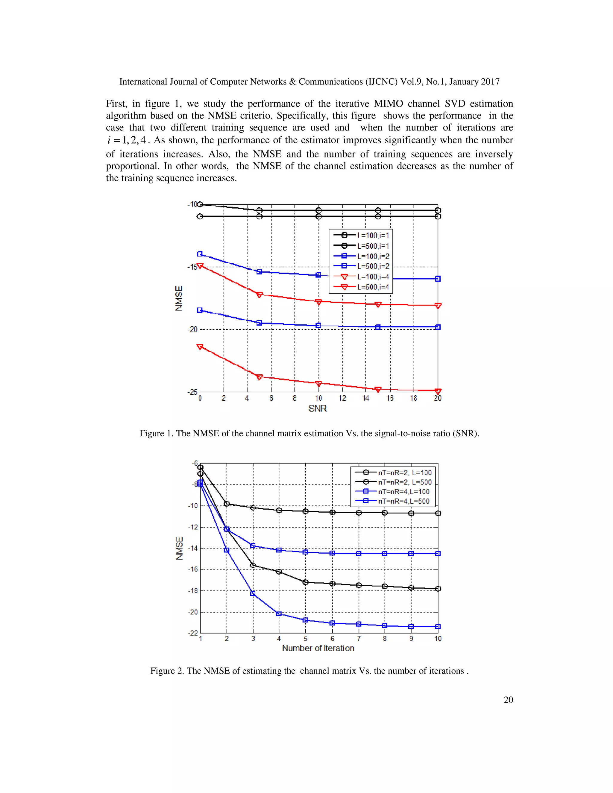
  International Journal ofComputer Networks & Communications (IJCNC) Vol.9, No.1, January 2017 21 Figure 2 shows the performance of the estimation algorithm as a function of the number of iterations and the number of receive antennas . This figure clearly shows that the performance improvement is insignificant after the 4th iteration. 6. CONCLUSIONS An introduction to the SVD has been introduced. The effect of using SVD in MIMO communication system has been discussed. It converts the MIMO system into parallel channel equal to the rank of the channel matrix, H . An iterative SVD technique is presented which is used to estimate the channel matrix from the transmit antennas to the receive antennas. Simulation results that show the effect of the number of transmit/receive antennas, the length of the training sequence and number of iterations on the performance of the presented iterative technique have been drawn. REFERENCES [1] I. E. Telatar, (1999) “Capacity of multi-antenna Gaussian channels”, European Trans. Telecommun., vol. 10, pp. 585–595. [2] A. Maaref and S. Aissa, (2008) “Capacity of MIMO rician fading channels with transmitter and receiver channel state information”, IEEE Trans. Wireless Commun., vol. 7, pp. 1687 –1698. [3] S. Jayaweera and H. Poor, (2003) “Capacity of multiple-antenna systems with both receiver and transmitter channel state information”, IEEE Trans. Info. Theory, vol. 49, pp. 2697 – 2709. [4] A. Zanella and M. Chiani, (2009) “Analytical comparison of power allocation methods in MIMO systems with singular value decomposition”, in IEEE Global Telecommun. Conference, pp. 1 –7. [5] S. Jin, X. Gao, and M. Mckay, (2006) “Ordered Eigenvalues of Complex Noncentral Wishart Matrices and performance analysis of SVD MIMO systems”, in ISIT, seatle, USA. [6] L. Garcia-Ordonez, D. Palomar, A. Pages-Zamora, and J. Fonollosa, (2005) “Analytical performance in spatial multiplexing MIMO systems”, in IEEE 6th Workshop on Signal Processing & Advances in Wireless Communications, 2005, pp. 460 – 464. [7] G. Lebrun, S. Spiteri, and M. Faulkner, (2004) “Channel estimation for an SVD MIMO system”, in IEEE Int. Conference on Commun., vol. 5, pp. 3025 – 3029. [8] Y. Tang, B. Vucetic, and Y. Li, (2005) “An iterative singular vectors estimation scheme for beamforming transmission and detection in MIMO systems”, IEEE Commun. Lett. , vol. 9, pp. 505 – 507. [9] A. Cano-Gutierrez, M. Stojanovic, and J. Vidal, (2004) “Effect of channel estimation error on the performance of SVD-based MIMO communication systems”, in 15th IEEE International Symposium on Personal, Indoor and Mobile Radio Communications, Vol. 1, pp. 508– 512. [10] G. Zamiri-Jafarian, H.; Gulak, (2005) “Iterative mimo channel svd estimation”, in Int. Confernce on Communications (ICC). [11] G. G. Raleigh and J. M. Cioffi, (1998) “Spatio-temporal coding for wireless communication”, IEEE Trans. Commun, vol. 46, pp. 357–366.