Gaussian curvature of implicitly defined surfaces

The scaling of {-3, 3} was inserted manually, because I didn't find a way to automate this. But this doesn't take too long. Start with {-1, 1} and go up or down.

Curvatures of implicitly defined surfaces

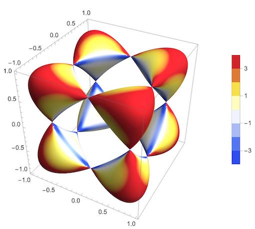
1. Gaussian curvature

The scaling of {-3, 3} was inserted manually, because I didn't find a way to automate this. But this doesn't take too long. Start with {-1, 1} and go up or down.

2. Mean curvature

The same link also provides a formula for Mean curvature:

fun = -x^2 + x^4 - y^2 + y^4 - z^2 + z^4; d1 = D[fun, {{x, y, z}}] // Simplify; d2 = D[fun, {{x, y, z}, 2}] // Simplify; mcur[x_, y_, z_] = Simplify[(d1 . d2 . d1 - Tr[d2] (# . # &[d1])) / (2 (# . # & [d1])^(3/2))]; Legended[ ContourPlot3D[fun == -1/2, {x, -1, 1}, {y, -1, 1}, {z, -1, 1}, ColorFunction -> Function[{x, y, z, u, v}, ColorData["TemperatureMap"][Rescale[Abs @ mcur[x, y, z], {0, 3}]]], ColorFunctionScaling -> False, Mesh -> False, PlotPoints -> 70], BarLegend[{"TemperatureMap", {0, 3.1}}, Automatic]] 

3. Mesh lines

The two curvature functions can also be applied to mesh lines:

fun = x^4 + y^4 + z^4 - (x^2 + y^2 + z^2)^2 + 3 (x^2 + y^2 + z^2); d1 = D[fun, {{x, y, z}}] // Simplify; d2 = D[fun, {{x, y, z}, 2}] // Simplify; mcur[x_, y_, z_] = Simplify[(d1 . d2 . d1 - Tr[d2] (# . # & [d1])) / (2 (# . # &[d1])^(3/2))]; Legended[ ContourPlot3D[fun == 3, {x, -2, 2}, {y, -2, 2}, {z, -2, 2}, ColorFunction -> Function[{x, y, z, u, v}, ColorData["TemperatureMap"][Rescale[Abs @ mcur[x, y, z], {0, 1}]]], ColorFunctionScaling -> False, Mesh -> 12, MeshFunctions -> Function[{x, y, z, u, v}, Rescale[Abs @ mcur[x, y, z], {0, 1}]], PlotPoints -> 70], BarLegend[{"TemperatureMap", {0, 1.1}}, Automatic]]