Analysis of the equation
It often is convenient to non-dimensionalize ODEs arising in physics, and this case is no exception. Rescale x and y by {x -> xn xs, y[x] -> yn[xn] ys}. Apply these transformations to the ODE, bringing the scale factors from the left side of the ODE, (xs^2/ys), to the right.
eqlast = (xs^2/ys) k ((e y[x]/c)^2 + 2 m*e y[x])^(3/2) /. y[x] -> yn[t] ys /. x -> xn xs /. t -> xn (* (k xs^2 (2 e m ys yn[xn] + (e^2 ys^2 yn[xn]^2)/c^2)^(3/2))/ys *)
Now, choose the scale factors, xs and ys, to eliminate the multipliers of yn[xn] and yn[xn]^2.
eq1 = eqlast[[1 ;; 3]] (eqlast[[4, 1, 1]])^(3/2) /. yn[xn] -> 1 /. xn -> 1 (* (2 Sqrt[2] k xs^2 (e m ys)^(3/2))/ys *) eq2 = eqlast[[1 ;; 3]] (eqlast[[4, 1, 2]])^(3/2) /. yn[xn] -> 1 /. xn -> 1 (* (k xs^2 ((e^2 ys^2)/c^2)^(3/2))/ys *) norms = FullSimplify[Solve[eq1 == 1 && eq2 == 1 && k > 0 && e > 0 && m > 0 && c > 0, {xs, ys}, Reals], k > 0 && e > 0 && m > 0 && c > 0] // Last (* {xs -> Sqrt[1/(c e k)]/(2 m), ys -> (2 c^2 m)/e} *)
Inserting these expressions into the transformed ODE yields,
eq = 1/xn D[xn yn[xn], {xn, 2}] == Simplify[eqlast /. %, k > 0 && e > 0 && m > 0 && c > 0] (* (2 yn'[xn] + xn yn''[xn])/xn == (yn[xn] (1 + yn[xn]))^(3/2) *)
which is somewhat easier to work with than the ODE in its original form. The question seeks a solution with very small y at large x. To obtain such an asymptotic solution, assume that y^2 is much smaller than y (in absolute value). Then, it is apparent that a solution exists equal to cf xn^a, a and cf constants.
Unevaluated[1/xn D[xn yn[xn], {xn, 2}] - (yn[xn] (1 + yn[xn]))^(3/2)] /. {(1 + yn[xn]) -> 1, yn[xn] -> cf xn^a} (* a (1 + a) cf xn^(-2 + a) - (cf xn^a)^(3/2) *)
For this expression to vanish, xn^(-2 + a) == xn^(3 a/2) clearly is required. In other words, a == -4. Then, cf is determined from
Simplify[% /. a -> -4, cf > 0 && xn > 0] (* -(((-12 + Sqrt[cf]) cf)/xn^6) *)
So, cf == 144, and this particular solution is yn[xn] == 144/xn^4. As we shall see, this is not the most general solution at large xn, but it does appear to be a separatrix.
Numerical Solution
With the constants given in the question, the scale factors become,
norms (* {xs -> 3.46944*10^-12, ys -> 1.022*10^6} *)
and the starting point of the integration, x0, normalized to xs, becomes (rationalized for future use in NDSolve)
x0n = Rationalize[x0/xs /. norms, 0] (* 723020393/5483051 *)
or about 131.865, and the specified value of y[x0], normalized to ys, becomes
y0n = Rationalize[10^6/ys /. norms, 0] (* 33547031/34284995 *)
or about 0.978476. Conveniently, x0n is well away from the singularity at xn == 0. The problem, now, is to choose yn'[x0n] to that yn[xn] approaches the separatrix, obtained above, at large xn. Employing a variant on the method employed to solve question 147207 yields the desired value of yn'[x0n].
xfn = 2000; s = ParametricNDSolve[{eq, yn[x0n] == y0n, yn'[x0n] == yp0, WhenEvent[Re@yn[xn] < 120/xfn^4 || yn'[xn] > 1/100, "StopIntegration"]}, yn, {xn, x0n, xfn}, {yp0, wp}, WorkingPrecision -> wp, AccuracyGoal -> Infinity, MaxSteps -> 20000];
WhenEvent[ ... ] is used here to terminate integration, whenever a numerical solution veers away from the separatrix. Doing so is desirable, because one hundred or more iterations at high WorkingPrecision typically are needed to obtain a desired solution. A small amount of experimentation is sufficient to determine that the initial value for yn'[x0n] is near -1.39. A better approximation then is obtained from
plt = Plot[Quiet@(yn[yp0, 15]["Domain"] /. s)[[1, 2]], {yp0, -1.306, -1.304}, PlotRange -> All]
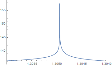
The improved estimate, given by the spike in the plot, is located within the range,
Cases[plt, Line[a__] :> a, Infinity] // Last; Position[%, Max[Last /@ %]][[1, 1]]; est = SetPrecision[{First[%%[[% - 1]]], First[%%[[% + 1]]]}, 45] (* {-1.30493508434085847547123648837441578507423401, -1.30493385315771526222761167446151375770568848} *)
This already narrow range is reduced much further with
dom[yp0_?NumericQ] := Quiet@(yn[yp0, 45]["Domain"] /. s)[[1, 2]] gg[bl0_, bu0_] := Module[{bl = N[bl0, 45], bu = N[bu0, 45], bt, db}, Do[bt = (bl + bu)/2; db = (bu - bl)/100; If[dom[bt] - dom[bt - db] > 0, bl = bt, bu = bt], {i, 120}]; bt];
(Note that FixedPoint could be used here instead of Do but appears to offer no advantage, at least for the present computation.)
r2000 = gg @@ est (yn[r2000, 45][xfn] /. s) - 120/xfn^4 (* -1.30493476864289837272478679314595905244023206 *) (* 8.3663144286145423790813208786836901834*10^-17 *)
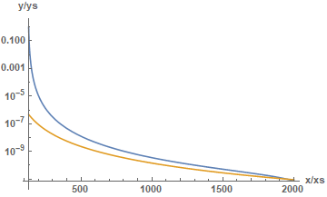
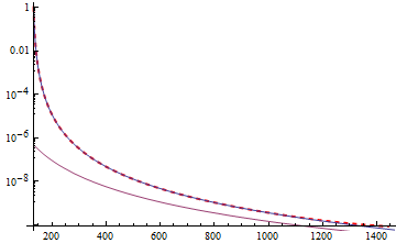
About 80 sec was used by my PC to obtain this result. Such very high precision usually is necessary when seeking a solution asymptotically approaching a separatrix. Below is a plot of the numerical result, in blue, and the separatrix, in orange.
LogPlot[{yn[r2000, 45][xn] /. s, 144/xn^4}, {xn, x0n, xfn}, AxesLabel -> {"x/xs", "y/ys"}, LabelStyle -> Directive[Bold, 11], PlotRange -> All]
As expected (and desired), the numerical solution is quite near the separatrix at large xn, even when viewed on a log plot.